R E S E A R C H
Open Access
Aircraft detection in remote sensing images
based on saliency and convolution neural
network
Guoxiong Hu
1,2, Zhong Yang
1*, Jiaming Han
1, Li Huang
3, Jun Gong
2and Naixue Xiong
4Abstract
New algorithms and architectures for the current industrial wireless sensor networks shall be explored to ensure the efficiency, robustness, and consistence in variable application environments which concern different issues, such as the smart grid, water supply, and gas monitoring. Object detection automatic in remote sensing images has always been a hot topic. Using the conventional deep convolution network based on region proposal for detection, there are many negative samples in the generated region proposal, which will affect the model detection precision and efficiency. Saliency uses the human visual attention mechanism to achieve the bottom-up object detection. Since replacing the selective search with saliency can greatly reduce the number of proposal areas, we will get some region of interests (RoIs) and their position information by using the saliency algorithm based on the background priori for the remote sensing image. And then, the position information is mapped to the feature vector of the whole image obtained by deep convolution neural network. Finally, the each RoI will be classified and fine-tuned bounding box. In this paper, our model is compared with Fast-RCNN that is the current state-of-the-art detection model. The mAP of our model reaches 99%, which is 12.4% higher than that of Fast-RCNN. In addition, we also study the effect of different iterations on model and find the model of 10,000 iterations already has a higher accuracy. Finally, we compare the results of different number of negative samples and find the detection accuracy is highest when the number of negative samples reaches 400.
Keywords:Remote sensing image, Detection, Saliency, Convolution neural network
1 Introduction
With the wireless sensor networks booming, various re-searches based on wireless sensor networks have made great progress [1–10], such as the physical sensors [11], architecture for the service computing [12], fault-tolerant optimization [13], data gathering and compres-sion [14], and smart data analysis [15]. Although the wireless sensor networks have been proposed, studied, and developed for more than a decade of years, there are still a lot of challenging issues especially in various in-dustrial scenarios [16, 17], including the object detection for the remote sensing images that are gathered by the industrial wireless sensor networks. We can obtain a large number of high resolution remote sensing images
obtained using various satellites and all kinds of sensors. For the object detection in these high-resolution remote sensing images, the traditional manual detection cannot meet the actual needs. Especially for the small target ob-jects in the image, it is hard to detect it quickly and ac-curately by artificial detection [18]. In the field of real-time image processing, automatic analysis and detection for remote sensing images will be highly cost-effective.
In the field of remote sensing image processing, it is of great military value for the automatic detection of air-craft in the airport [19]. The texture, color, and other characteristics of aircraft are very similar to those of the background in the remote sensing image because the airports are often built in desert or remote spaces, where the color is single and often gray [20]. It often fails to detect the aircraft using a general automatic detection method based on low-level image features. Later, the re-searchers have introduced the machine learning method
* Correspondence:[email protected]
1College of Automation Engineering, Nanjing University of Aeronautics and
Astronautics, Nanjing 211106, China
Full list of author information is available at the end of the article
into the field of remote sensing image automatic detec-tion, good results have been achieved. Considering the implementation principle, algorithms for aircraft recog-nition can be briefly summarized in three categories. The first category is mainly based on statistical feature learning method. It usually constructs rotation-invariant and scale-invariant features based on shape, texture, and geometric features. These features include Hu moments [21], Zernike moments [22], wavelet moments [23], the Fourier descriptor [24, 25], and sift [26], which are ac-companied by the generally adopted classifiers, e.g., SVMs and neural networks.
The second category is the template matching method for aircraft detection. Considering that the size and shape of the aircraft is similar between the same types of aircraft, researcher design the various shape templates for each type of aircraft and compute a similarity meas-urement between the template and aircraft. In [27], the authors propose a template-matching method using high-level features of aircraft shape. The method inte-grates a coarse-to-fine process. The first coarse stage is the rough estimation phase. In this stage, the estimation score is given according to the matching degree of the single type of aircraft. The second fine stage is the re-finement stage. In this stage, the aircraft shape parame-ters are obtained by using the combined features and kernel functions. In [28], Wu et al. propose a robust air-craft detection method without the shape and silhouette extraction of the aircraft. The authors firstly apply a dir-ection estimation method to align the aircraft to the same direction for further matching and employed a re-construction similarity measure to transform type recog-nition into a reconstruction problem. Then, a jigsaw matching pursuit algorithm is proposed to solve the re-construction problem. Although the template-matching method is easy to implement, there are also the follow-ing problems [29]:
(1)The template-matching method is only applicable to the rare samples or low resolution images. If the resolution of the image is higher or the image size is larger, more feature points will be generated, which result in slower matching. If the number of tem-plates for the target sample is larger and all these templates are matched one by one with the samples in images, the computation is very large and it is dif-ficult to guarantee the speed of calculation. If only a few of the samples are selected as the reference sam-ples, it leads to uncovering all features of the sample and waste of information resources. Meanwhile, how to select target samples is also a difficult point. (2)Remote sensing image is photographed in complex
environments, which not only includes light, viewpoint, and scale variant but also includes the
influence of atmospheric and cloud cover, complex background, and similar ground environment. These disadvantages cause images blurring. The insufficient samples and obvious difference between the
templates and the identified images will lead to detection accuracy decreased even a failure to match.
(3)The traditional method of object detection based on feature matching can only detect and recognize one type object by a given template, but cannot model and classify multi type objects at the same time.
The last category is deep learning. Since 2012, Hinton [30] gets significant achievements in the ImageNet clas-sification using the deep learning algorithm: the deep learning methods have achieved very good results in various fields such as object classification and recogni-tion. In 2014, Girshick et al. proposed the RCNN [31] that first uses depth convolution neural network for ob-ject detection. The authors first use selective search [32] to extract the region proposal from the original image, and then use the multi-layer convolutional neural net-work to extract the features of objects in the region pro-posal. Finally, SVM or softmax is used for classification and positioning. The method achieves the best effect of the object detection in that year.
The authors have applied this method to aircraft de-tection in remote sensing images since the depth learn-ing has higher accuracy in object detection field. But there are so many region proposals, about 2000, ex-tracted by the RCNN algorithm [31] using the selective search [32]. Extracting features from so many region proposals using convolution network will result in very low efficiency. In addition, in the 2000 region proposals, only a very small number of them are regions of interest (RoIs), and most of the regions are background. So many negative samples in the classification will affect the de-tection accuracy.
it computes three saliency maps using center-surround differences, which are combined together to form the final master saliency map. Later, a lot of research efforts have been made to design various saliency features char-acterizing salient objects or regions.
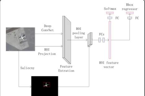
If the saliency algorithm is used to preprocess the image, it can greatly reduce the number of region pro-posals and improve the efficiency and accuracy of subse-quent feature extraction and classification because the saliency algorithm can quickly find detected objects in the image. In this paper, we first get some region pro-posals by using the saliency algorithm to preprocess the original image. Then, the bounding box of these region proposals are obtained by thresholding calculation and connected domain method. The area that the bounding box contains is the RoI that we need to be detected. Fi-nally, the Fast-RCNN [34] model is used to extract, map, and classify these RoIs, and the final test result is ob-tained by region proposal regression operation. As Fig. 1 shows, our detection network takes as input an entire image and a set of object proposals that are obtained with the saliency algorithm. The network first processes the whole image with several convolutional and max pooling layers to produce a conv feature map. Then, for each object proposal a region of interest pooling layer extracts a fixed-length feature vector from the conv fea-ture map. Each feafea-ture vector is fed into a sequence of fully connected (fc) layers that finally branch into two sibling output layers: one that produces softmax prob-ability estimates over “aircraft” class and “background” class and another layer that outputs four real-valued numbers, which encode refined bounding-box positions for each of the“aircraft”class.
It is obvious that the aircrafts area is small in propor-tion to the whole image and the color and texture fea-tures of the aircrafts are similar to those of the background in the remote sensing image. So it usually leads to low accuracy using the conventional saliency
algorithms, i.e., saliency algorithm based on regions and saliency algorithm based on frequency, to calculate the salient map because many small planes are filtered out as background chip. In [35], the robust saliency algo-rithm based on background priors can solve this prob-lem. However, the algorithm uses statistical object area method, which is very difficult to calculate because the target object is irregular shape in images, to compute sa-lient objects. Our algorithm uses statistical pixel number instead of statistical area method based on [35]. Experi-ment shows that this method can achieve good results. In addition, our algorithm is also compared with the state-of-the-art algorithms, e.g., IT [33], HC [36], RC [36], FT [37], CA [38], LC [39], SR [40], DSR [41], BL [42], and our saliency algorithm has good robustness to the remote sensing image.
We also compare our object detection model, which combined saliency algorithm with depth detection algo-rithm, and the state-of-the-art detection model. Our model gets higher recognition rate and detection accur-acy than the latter.
The paper is organized as follows:. in Section 2, we introduce related works. Thereafter in the Section 3, we demonstrate the saliency algorithm based on back-ground priori and the detection network. Experiments are presented in Section 4. We conclude with a discus-sion in Section 5.
2 Related works
the local contrast methods, so that the entire saliency area cannot be significant.
Considering the disadvantages of computing saliency image using local contrast, we can obtain the saliency image using global contrast method. Zhai and Shah et al. [40] use the MZ algorithm to calculate the contrast of each pixel in the whole image. Inspired by this, Fenget et al. [48] used the sliding window to calculate the global contrast. Margolin et al. [49] obtain the saliency of image blocks by using the statistical information of image and linearly fusing the color contrast of image blocks.
Cheng et al. [37], calculate the histogram contrast of the whole image to obtain the saliency image. It means the wider the distribution of a color in the image, the lower the probability of the saliency region that contains this color. The color space distribution can be used to describe the salient area.
A color is more widely distributed in the image and the probability of the saliency including this color is smaller. So, the special color space distribution can be used to describe the saliency region. Perazzi et al. [50] obtain saliency image by computing the variance of each super-pixel’s color spatial distribution, which is got by the adaptive super-pixel segmentation method. The glo-bal contrast method, which calculates the whole image, will produce a saliency image of uniform density. How-ever, the computational complexity increases using the global image processing. And if reducing the resolution or reducing the feature dimension is applied to address the problem, it leads to minutiae deletion and sensitive to noise.
Both local contrast and global contrast methods be-long to the airspace mode. In order to improve the ro-bustness of model and improve the checking efficiency of model, some people transform the image from the spatial domain to the frequency domain for calculating image contrast. Hou et al. [41] find that there are some similar spectrums among the similarity images in fre-quency domain. Based on it, Hou et al. propose a spec-tral residual method to compute salient image. The detail of the method as follows. Firstly, the original image is transformed from spatial domain to frequency domain. Then, the amplitude spectrum, phase spectrum, and amplitude spectrum residuals are computed in the frequency domain. Finally, the final saliency image is ob-tained by inverse Fourier transform. Different from Hou’s analysis of amplitude spectrum, Guo et al. [51] get the saliency image by analyzing phase spectrum. Achanta et al. [38] find that the high frequency part of the image reflects the overall information of the image, and the low frequency part reflects the detail informa-tion of the image. That is, the saliency image is larger probability in low frequency.
In addition, with the wide application of deep learning in recent, it achieves a good result by introducing the depth learning method into the computation of saliency image. Li et al. [52] get the saliency image by calculating the contrast of high-level features that are extracted from three different scale images by the CNNs (deep convolutional neural networks). Zhang et al. [53] think that it cannot obtain a saliency image accurately in spatial domain if the original image has low resolution, and the features of the image are extracted totally dependent on CNNs. So they propose the saliency model based on CNNs of spatial-temporal.
The traditional object detection method uses a sliding window to divide an image into millions of sub windows with different positions and scales, and then, each sub window is determined by the classifier whether it is the target object.
Traditional methods use a sliding window frame to break down an image into millions of sub-windows with different locations and different scales, and then use the classifier for each window to determine whether the tar-get object is included. For each type of object, traditional methods extract its unique features and design specific classifiers, e.g., face detection algorithm is usually Haar feature +Adaboosting classifier [54]. Pedestrian detection algorithm is HOG feature (histogram of gradients) + SVM (support vector machine) [55]. And the detection algorithm of general objects is the HOG feature +DPM (deformable part model) [56, 57].
Recently, most of object detection algorithms are based on the deep learning frameworks. These algo-rithms are mainly classified into two groups: one is ob-ject detection method based on region proposal [58–60], which is a mainstream algorithm, e.g., RCNN [31], SPP-Net [61], Fast-RCNN [34], Faster-RCNN [62], and MSRA recently proposes algorithm R-FCN [63]. The other is not using the region proposal method to detec-tion, e.g., YOLO [64] and SSD [65].
speed of calculation because the feature extraction cal-culations of different RoI can be shared.
Whether it is SSP-Net or Fast-RCNN, although they re-duce the number of CNN operations, still need to gener-ate the region proposal box for each image using selective search, which takes 2 s/image. The time consumption of selective search on the CPU is far greater than that of the CNN on the GPU. Therefore, the bottleneck of object de-tection is the region proposal operation.
In order to save selective search operating time, Faster-RCNN inputs the convolution feature of the image to the RPN (region proposal network) layer and obtains the region proposal. After the RPN layer, the re-gion proposal is required to be categorized and fine-tuned through softmax classifier and bounding box. Ex-periments show that Faster-RCNN is not only more fas-ter but also has higher detection accuracy. Considering the full connection operation is also a time-consuming process of RoIs in Faster-RCNN, R-FCN Faster also in-corporates this process, which shares computing for dif-ferent RoIs, into the forward computation of the network. So R-FCN is faster than Faster-RCNN.
The latter object detection method does not use re-gion proposal for object detection. YOLO divides the original image into S*S cells. If the center of an object falls into a cell, the corresponding cell is responsible for detecting the object and gives confidence score for each cell. The score reflects the possibility of the target object and the accuracy of location of the target predicted by bounding box. Since YOLO did not use the region pro-posal, but directly conduct convolution operation on the image, it is much faster in detection than Faster-RCNN but the accuracy is less than that of Faster-RCNN. SSD also uses a single convolutional neural network to con-volute the image, and predicts a series of bounding boxes with different sizes and aspect ratios at each pos-ition of the feature vector. During the testing phase, SSD predicts the possibility that each bounding box contains objects is a target object and adjusts the bounding box of the object to accommodate the size. G-CNN [67] regards the object detection as a process of changing size of the bounding box from fixed cell to the real bor-ders of the object. Firstly, SSD divides the whole image
into some cells with different size to obtain the initial detection bounding box and convolutes the whole image to get a feature vector of it. Then, the feature vector cor-responding to the initial bounding box is transformed into a fixed-size feature vector by Fast-RCNN. Finally, a more accurate border of the target object is got through a regression process.
In short, the performance of the first type of detection is better, but slower, while that of the other is slightly worse, but faster [68]. Recently, some researchers carry out the object detection from other perspectives. For ex-ample, many researchers regard that the lower layer of the neural network usually retain more fine-grained, while the higher layer of it usually has better semantic features. To improve the accuracy of detection, the fea-tures of different layer are fused [59] [69–73]. Other re-searchers combine the object detection with other applications of image processing, e.g., Kaiming [74] com-bine the object detection with image segmentation and gets good results.
3 Model introduction
In order to obtain an efficient and robust detection model, we change the selective search method of Fast-RCNN to a more efficient saliency method. Since the sa-liency method has fewer region proposals and more ac-curate location, the computation of bbox regression is reduced in followed Fast-RCNN. In addition, it improves accuracy of detection because of reducing the number of negative samples. As Fig. 2 shows, the algorithm consists of two parts: region proposal and object detection net-work. The region proposal mainly generates some object proposals with the saliency algorithm, and the object de-tection network carries out the dede-tection function of the object based on Fast-RCNN. Our algorithm firstly pro-cesses the whole image with several convolutional and max pooling layers to produce a conv feature map. Then, for each object proposal that is generated with the saliency algorithm a RoI pooling layer extracts a fixed-length feature vector from the conv feature map. Each feature vector is fed into a sequence of fully connected (fc) layers that finally branch into two sibling output layers: one that produces softmax probability estimates
over aircraft class and background class, another layer outputs the bounding-box positions for each of the air-craft. The algorithm flowchart is shown in Fig. 2.
3.1 Region proposal acquisition
Currently most of the models use the selective search method to obtain region proposals, which solves the time-consuming and resource problems caused by the previous exhaustive search method. The method includes two steps. Firstly, 1000 ~ 3000 region proposals are randomly gener-ated in an image. And then, these region proposals are merged through certain strategies, e.g., similarity measures of texture or color. The selective search method has a good result on the images with gradation distinction of clear color or texture feature. However, for objects such as aircrafts, whose features have similar background features in the re-mote sensing image, the effect is poor.
In addition, Fast-RCNN obtains about 2000 RoIs that include target objects and non-target objects method. Most of these RoIs are negative samples, which not only reduce the detection efficiency, but also reduce the de-tection accuracy. For this problem, we propose using sa-liency method to calculate the RoIs whose number is much smaller than those of Fast-RCNN.
But the common saliency methods are often fail to high-quality saliency image due to the small size of the aircraft in the remote sensing image. In [18], researchers obtain the saliency image through the recognition of the foreground based on background prior. The method proposed in the paper [35] mainly to determine whether the object is a sali-ency object by the ratio of the area of target object to the area of the part connecting to the image boundary. But be-cause remote sensing image has low resolution and the size of object is small, it cannot calculate the area of object and fails to generate the saliency image for small object. Our al-gorithm calculate saliency image by counting the number of pixels of target object and those of the part connecting to the image boundary based on background prior pro-posed in [35]. Specific implementations are as follows:
(1)Background perception
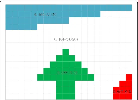
We observe that object and background regions in images are quite different in their spatial layout, i.e., object regions are much less connected to image boundaries than background ones. As shown in Fig.3, there are four regions: blue, white, red, and green. The blue region and white region are the backgrounds since they significantly touch the image boundary. Only a small amount of the red region touches the image boundary, but as its size is also small, so it looked as a partially cropped object. The green region is clearly a salient object as it is large, compact, and only slightly touches the image boundary.
(2)We can obtain salient objects by the ratio of the number of pixels of the part touching the image boundary to those of the entire object field. The part with the smallest ratio is the salient object as shown in Eqs. (1)~(3).
BndConð Þ ¼p NumPixelð Þp
TotalPixelð Þp ; ð1Þ
NumPixelð Þ ¼p fpjp∈R;p∈Bndg; ð2Þ
TotalPixelð Þ ¼p fpjp∈Rg; ð3Þ
wherepis an image pixel,Ris an object region, and Bnd is the set of image boundary pixels.
(3)Pixel calculation
Because it is difficult to segment the image
accurately, it is difficult, in the practical application, to count the number of pixels of the part touching the image boundary and the total number of pixels of the entire object. We use super-pixel instead of pixels. Firstly, the superpixels are obtained using SLIC [75], and then, we calculate the shortest path between all adjacent superpixel to construct similar-ity of them as in Eq. (4).
dgeoðp;qÞ ¼ min
p1¼p;p2;…;pn¼q Xn−1
i¼1
dapp pi; ;piþ1
; ð4Þ
Where dgeois the shortest path between superpixel p and superpixelq. For convenience, we definedgeo(p,p) =
0.Finally, Eq. (5) computes the number of superpixels of the region that superpixelpbelongs to.
TotalPixelð Þ ¼p X
n
i¼1
exp −d
2 geoðp;piÞ
2σ2 clr
!
¼Xn
i¼1
S pð ;piÞ; ð5Þ
where n is total number of superpixels. We use the Gauss function to map the similarity of two superpixels to (0, 1]. Whenpiis similar top,dgeo= 0ands= 1, which ensures the number of super pixels increases 1 when p
and pi are similar. Otherwise, On the contrary, when p
and pi are not similar, i.e.,dapp(∗,∗) > > 3σclr, s=
0.Simi-larly, the number of pixels touched the boundary can be obtained as in Eq. (6).
NumPixelð Þ ¼p X
n
i¼1
S pð ;piÞ δðpi∈BndÞ; ð6Þ
whereδis 1 for superpixels on the image boundary, and 0 otherwise. In experiment, we take 200 superpixels for a typical 300 × 400 resolution image and find that the ef-fect reaches best whenσclris 10.
(4)Algorithm updating
In order to ensure that the saliency objects can be completely segmented, we regard the partially cropped objects, which are located in the middle of the image and untouched the image boundary, as the saliency objects, i.e., NumPixel(p) = 0 and TotalPixel(p) are relatively small. This method can guarantee the number of negative samples, which improve training accuracy of the following object detection model, while not missing the real objects.
3.2 Object detection model
Girshick proposed a RCNN model for object detection in 2014 and achieved the best detection results in that year. The RCNN firstly uses selective search method to
generate many region proposals (RoIs), and then uses CNNs to extract feature of each RoI. Finally, the RoIs are classified and its bounding boxes are regressed by the softmax classifier and bbox regressor. The RCNN has the very low detection efficiency because about 2000 RoIs produced by selective search are extracted feature by CNNs. Later, Girshick proposed the Fast-RCNN model based on the RCNN. That model firstly extracted the feature of whole image using CNNs. Then, the 2000 RoIs are mapped the feature vector according to the bounding box of those RoIs, and do not extract its fea-tures. Since the feature extraction operation is carried out only one time during the whole detection period, the detection efficiency has been greatly improved. The detection accuracy of Fast-RCNN is lower because most of them are negative samples in 2000 RoIs. As shown in Fig. 4, we use saliency method to produce some saliency objects as the RoIs and send these RoIs into detection network to detect objects. The detection network ex-tracts the feature of the whole image by five CNN layers and some pooling layers. And then, the bounding box of the saliency object is mapped to this feature vector in RoI pooling layer. Finally, the saliency object is classified and its bounding box is regressed.
(1)RoI pooling layer
The bounding box information of RoIs produced by saliency method mainly consists of a four-tuple (r,c,
h,w) that specifies its top-left corner (r,c) and its height and width (h,w). In addition, since the area of RoIs is any size, we divide theh × wRoI intoh/
7 × w/7sub-regions of 7×7 size for calculation
con-venience. Then, max-pooling the values in each sub-region into the corresponding output grid cell. The RoI pooling layer is simply the special-case of the only one spatial pyramid pooling layer used in SPPnets [22].
(2)Fine-tuning
In the back-propagation, the traditional detection networks, e.g., RCNN or SPPnets, are highly
inefficient because the number of RoIs is large and the entire image also is processed when each RoI needs to be retrained.
Our method based on Fast-RCNN uses a share par-ameter way, which shares the feature between back-propagation networks and forward pass by stochastic gradient descent (SGD), during training. Fast-RCNN has proved the hierarchical sampling method (i.e., each batch data contains 2 images and 128 RoIs for each image) is effective during training. However, due to the fact that the number of RoIs produced by the saliency method is small and there are less than 128 ROIs in each image, we combine two types of RoIs, one of which is obtained by the saliency algorithm and the other is randomly generated, to improve the detection accuracy in the actual training process. In addition to the hierarchical sampling, Fast R-CNN uses a streamlined training process with one fine-tuning stage that jointly optimizes a softmax classifier and bounding-box regressors, rather than training a softmax classifier, SVMs, and regressors in three separate stages. Our method also adopts this method to improve efficiency.
(3)Loss function
There are two output layers in the detection model: one output is used to describe the probability distribution of each RoI,p= (p0,p1,…,pu), andpis computed by a softmax over theu+ 1 outputs of a fully connected layer. Since we detect only one type of object in remote sensing image, so we setu= 1. The other output layer is the bounding box
regression offsets,tu= (txu,tuy,twu,thu), for each of theu object classes, indexed byu.tuspecifies a scale-invariant translation and log-space height/width shift relative to an object proposal.
Each training RoI is labeled with a ground-truth classuand a ground-truth bounding-box regression targetv. We use a multi-task loss functionL:
L pð ;u;tu;vÞ ¼Lclsðp;uÞ þλ½u≥1Llocðtu;vÞ; ð7Þ
where Lcls(p,u) = −logpu is the log loss of the real cat-egory u. The second regression loss function Lloc is the
loss between the real object position informationv= (vx,
vy,vw,vh) and the predicted object position informationtu = (txu,tyu,twu,thu). The super parameter λ balances two loss function, and we takeλ= 1 in the experiment.
Experiment shows that, for remote sensing images,
L1regularization is better thanL2regularization, so we useL1smoothing loss function forLloc:
Llocðtu;vÞ ¼
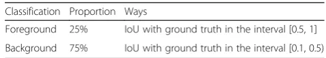
During fine tuning, we enter two images every time, randomly select 64 RoIs for each image. We take 25% of the RoIs from object proposals that have intersection over union (IoU) overlap with a ground truth bounding box of at least 0.5. These are the positive samples, i.e.,u> = 1. The remaining RoIs are sampled from object proposals that have a
maximum IoU with ground truth in the interval [0.1, 0.5). These are the negative samples, i.e.,u= 0. The lower threshold of the negative sample is 0.1 because of a heuristic for hard example mining. During training, the image has a probability level of 0.5 to flip. The table of sample allocation is shown in Table1.
(5)Scale-invariance
Fast-RCNN explores two ways of achieving scale invariant object detection: (1) via“brute force” (single-scale) learning and (2) by using image pyramids (multi-scale). A single-scale directly pre-defined pixel size during both training and testing. The network must directly learn scale-invariant ob-ject detection from the training data.
During multi-scale training, we randomly sample a pyramid scale each time an image is sampled, and then train the image object with an approximate scale invariant sampled. At test-time, the image pyramid is used to approximately scale-normalize each object proposal.
Experiment of Fast-RCNN shows that the mAP of single-scale is lower 1.2 to 1.5% than that of multi-scale for the AlexNet and VGG_CNN_M_1024 model, but the former is faster than the latter in terms of detection speed.
So we can see that the deep neural network is not sensitive to the scale of the object. Multi-scale image is only slightly higher in detection accuracy than a single-scale image, but the efficiency is greatly re-duced. Therefore, we use the single-scale approach (i.e., the short edge is limited to 300 pixels, the long edge is limited to 500 pixels) to training and testing the image.
(6)Object detection
Once the detection network is fine-tuned, the detec-tion amounts to little more than running a forward
Table 1The table of sample allocation
Classification Proportion Ways
Foreground 25% IoU with ground truth in the interval [0.5, 1]
pass. The network takes as input an image and a list of RoIs to score. During the testing phase, all 400 RoIs will be scaled to 224×224 pixels when the image pyramid is used to extract the features of the RoIs.
For each test RoIr, the network outputs a posterior probability distributionpand a series of predicted bbox offsets relative tor(each of the u classes gets its own refined bounding-box prediction). Then, we assign a detection confidence torfor each object
classuusing the estimated probabilityPr(class =u|
r) =Pu. Finally, we perform non-maximum suppres-sion independently for each class.
4 Experiments
4.1 Data set acquisition
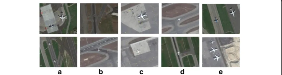
We sample 1200 images containing the aircraft from google earth, and the resolution of each image is be-tween 300 ×300 pixels and 700 × 700 pixels. Since the airport is in the remote places, there are three main
a
b
c
d
e
types of background: grassland, land, and cement. As shown in Fig. 4, to ensure data sets cover all types of data, we sample lots of samples from those different backgrounds. Besides, in our data set, there are some images containing a different number of aircraft: one is the image with a single aircraft, and the other is with multiple aircrafts.
4.2 Saliency experiment
We compare our algorithm with the state-of-the-art sali-ency algorithms, e.g., IT [33], HC [36], RC [36], FT [37], CA [38], LC [39], SR [40], DSR [41] and BL [42] in the five types of data set. IT is the most cited algorithm. HC calculates saliency image based on global histograms. RC obtains saliency image based on local contrast method. CA combines local contrast with global contrast to cal-culate saliency image. FT calcal-culates saliency image in the frequency domain. LC uses the combination of time do-main and frequency dodo-main to obtain saliency image. SR calculates it in frequency domain. And BL adopts the machine learning method for saliency image. In the ex-periment, all of algorithms employ the source provided by the author except the LC using the program provided by the paper [36] because its author did not provide
source code. Running results of all algorithms in differ-ent types of image set are shown in Fig. 5. IT is the earli-est to use computer to simulate the biological visual attention mechanism, which mainly contrasts the color, brightness and direction of the image with the back-ground to get a saliency image. The result of IT is the ef-fect to be bad actually because of the similarity between the background color, texture, and brightness in remote sensing image. The HC algorithm, which is proposed a global histogram method, cannot obtain the better sali-ency image based on global histogram due to the worse discrimination of the color feature in remote sensing image. RC, relative to the HC, uses local contrast to ob-tain a saliency image, and the effect is better than that of HC in the all types of background except grassland. CA combines the global and local contrast methods, which can distinguish between background and foreground. But from Fig. 5, it is difficult to obtain a high quality binary image through a suitable thresholds, CA can not accurately box the aircraft objects.
The other algorithms different from the past in the time domain, e.g., FT, etc., achieve a better saliency image in the frequency domain except the small objects in remote sensing image as shown in Fig. 5b. Through the above analysis, we can see that the conventional sali-ency algorithms cannot receive better results only by local contrast calculation, global contrast calculation, or biological vision-based saliency calculation because the remote sensing image has the characteristics of low reso-lution, the small target object, and low color contrast be-tween foreground and background. Our algorithm, Table 2The mAP with different iteration time
Method Iteration number
10,000 20,000 30,000 40,000
Fast rcnn 0.84 0.855 0.847 0.866
Our algorithm 0.97 0.981 0.91 0.99
according to the object area accounts for a large propor-tion of the whole image as the background and the re-mains is foreground, has better robustness for remote sensing image processing based on background prior.
To obtain objects with bounding boxes, we need to box the saliency image after obtaining the saliency image. Since the foreground has been separated from the background when we get the saliency image, a sple connected domain method can box the saliency im-ages. And to ensure the entire aircraft can be boxed, the overlapping bounding box is merged according to the maximum principle of merger.
RCNN, Fast-RCNN, and Faster-RCNN are currently the state-of-the-art three object detection methods. The first two methods, i.e., RCNN and Fast-RCNN, will
generate about 2000 RoIs during the object detection and the last method also generates at least 300 RoIs. However, as shown in Fig. 6, these RoIs, whose number is smaller than 2000 RoIs that obtained by Fast-RCNN, are put into detection network to train model and the training model time is much smaller than it by Fast-RCNN.
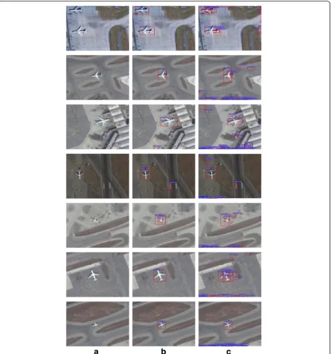
4.3 Object detection
We compare our algorithm with Fast-RCNN in this sec-tion. Fast-RCNN firstly obtains 2000 RoIs using selective search, and then the bounding box information of those RoIs are mapped to feature vector of the whole image by CNNs. Finally, these RoIs are classified by softmax and its bounding boxes are fine-tuned by bbox. To analyze
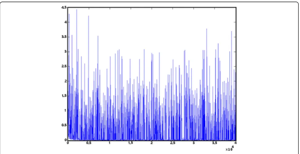
Fig. 8Loss presented the state of dispersing
a
b
the influence of the number of iterations on model checking effect and training time in CNNs, we compare mAP with the different number of iterations.
As shown in Table 2, the more the number of training, the greater the mAP, which is consistent with the basic theory of deep convolution network. In addition, we also can find that the mAP of our network is about 10% higher than that of Fast-RCNN from the above Table 2.
The loss chart of training of the two algorithms is shown in Fig. 7.
As shown in Fig. 7, we can find that the loss rate is ba-sically stable when the number of iterations reached 10,000 and the average loss rate is only reduced about 1% when the number of iterations is increased to 30,000. So, we can use the model of 10,000 iterations to detect object in the real-time application.
The saliency method, which can highlight the suspect object to generate RoIs in image preprocessing, is com-pletely different from the Fast-RCNN. The threshold has a great influence on the number of salient objects during using saliency method to generate the salient maps. Al-though we adjust the different thresholds as much as possible to minimize the impact, the total number of RoIs in each remote sensing image is still small and the number of negative samples is less in such a small amount of RoIs. To examine the effect of different num-ber of negative samples on the detection accuracy, we compare the results obtained with the different number of negative samples in experiment. Firstly, we directly put the RoIs that are generated by saliency algorithm into network to train and find the loss rate shows a di-vergent state (shown in Figure 8). So the trained model fails to detect objects.
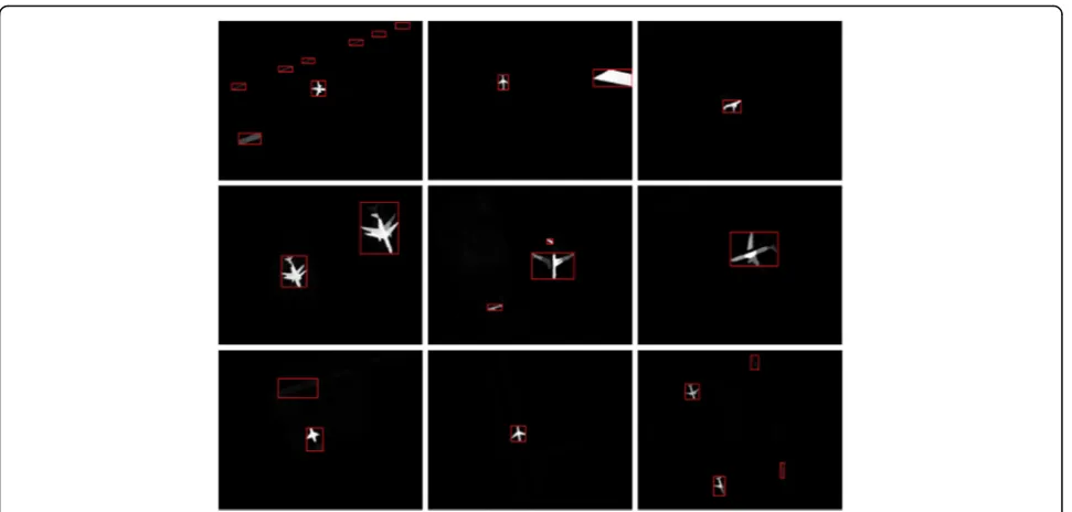
Then, we randomly generate 200 and 400 RoIs for sali-ency processed images respectively. To ensure all of gen-erated RoIs are negative samples, those that overlapping reaches 50% with the original RoIs will be discarded. Fig-ure 9 shows the result of different number of negative samples. The detection effect and the calibration accur-acy of the bounding box have been very accurate when the negative samples increase to 400. Many objects that belong to the background image are labeled as target ob-jects, and some bounding boxes of objects are boxed in-accurately because the number of negative samples is low that leads to model training inadequate.
5 Results and discussion
Since the RoIs generated by saliency method are less than those generated by select search method, our algo-rithm can greatly improve the detection precision and reduce the detection time than the other state-of-the-art algorithms, e.g., RCNN, Fast-RCNN, and Faster-RCNN. But our saliency algorithm based on background prior has a poor effect when the boundaries are fuzzy between the foreground and the background, so it is difficult to obtain some clear salient map if the boundaries are fuzzy, which leads to failure of subsequent object detection.
6 Conclusions
Since remote sensing images have low resolution and the target objects in it are very small, the conventional automatic object detection method is very difficult to de-tect objects accurately. The current object dede-tection al-gorithm based on deep learning is required to obtain a large number of RoIs, and most of those RoIs are nega-tive samples. These redundant neganega-tive samples not only reduce the detection accuracy, but also increase the training time of the model. We propose a very robust and efficient detection method by combining
background prior-based saliency detection algorithm with the CNNs based object detection algorithm.
For future work, we believe that investigating more so-phisticated techniques for improving the saliency accur-acy, including the deep convolution neural network, will be beneficial. Moreover, since it is a time-consuming for fitting parameters of model, we propose the share fea-ture method between saliency detection and object de-tection using CNNs in order to further improve the efficiency of model training.
Acknowledgements
Thanks are due to Xingxing Huang and Lingfeng Hu for the assistance with the experiments.
Funding
This work was supported by the National Natural Science Foundation of China under grant no. 61473144, 41661083, 61602222, 61562044; Aeronautical Science Foundation of China (Key Laboratory) under grant no. 20162852031; the special scientific instrument development of Ministry of Science and Technology of China under grant no. 2016YFF0103702; The National Science Foundation of Jiangxi Province under grant no. 20171BAB212014.
Availability of data and materials
We sample 1200 images containing the aircraft from google earth, and the resolution of each image is between 300×300 pixels to 700 × 700 pixels. Since the airport is in the remote places, there are three main types of background: grassland, land, and cement. To ensure data sets cover all types of data, we sample lots of samples from those different backgrounds. Besides, in our data set, there are some images containing a different number of aircraft: one is the image with a single aircraft, and the other is with multiple aircrafts.
Authors’contributions
GH contributed in the conception and design of the study. ZY carried out the simulation and revised the manuscript. JH and JG helped to perform the analysis with constructive discussions. Meanwhile, LH was responsible for producing simulation analysis and writing the manuscript carefully. Furthermore, NX went through and approved the final manuscript. All authors read and approved the final manuscript.
Authors’information
Guoxiong Hu is currently a doctoral student at College of Automation Engineering, Nanjing University of Aeronautics and Astronautics, China. He works at Jiangxi Normal University, China. Currently, he majors research fields including pattern recognition, image processing, and deep learning. Zhong Yang, he is a professor and doctoral supervisor at College of Automation Engineering, Nanjing University of Aeronautics and Astronautics, China. He has published about more than 100 research papers (including about 30 SCI/EI-indexed papers). He currently majors research fields including robot control and pattern recognition.
Jiaming Han is currently a doctoral student at College of Automation Engineering, Nanjing University of Aeronautics and Astronautics, China. He currently majors research fields including pattern recognition, image processing, and deep learning. Li Huang is currently a doctoral student at School of Information Technology, Jiangxi University of Finance and Economics, China. She works at Jiangxi Normal University, China. She currently majors research fields including information management and knowledge management. Jun Gong is a teacher in the College of Software, Jiangxi Normal University, Nanchang, China. And he earned the PhD degrees from Wuhan University, Wuhan, China in 2016.
University, Wentworth Technology Institution, and Colorado Technical University about 10 years. His research interests include Cloud Computing, Security and Dependability, Parallel and Distributed Computing, Networks, and Optimization Theory.
Dr. Xiong published over 280 international journal papers and over 120 international conference papers. Some of his works were published in IEEE JSAC, IEEE or ACM transactions, ACM Sigcomm workshop, IEEE INFOCOM, ICDCS, and IPDPS. He has been a General Chair, Program Chair, Publicity Chair, PC member and OC member of over 100 international conferences, and as a reviewer of about 100 international journals, including IEEE JSAC, IEEE SMC (Park: A/B/C), IEEE Transactions on Communications, IEEE Transactions on Mobile Computing, IEEE Trans. on Parallel and Distributed Systems. He is serving as an Editor-in-Chief, Associate editor, or Editor mem-ber for over 10 international journals (including Associate Editor for IEEE Tran. on Systems, Man, and Cybernetics: Systems, Associate Editor for Information Science, Chief of Journal of Internet Technology (JIT), and Editor-in-Chief of Journal of Parallel and Cloud Computing (PCC)), and a guest editor for over 10 international journals, including Sensor Journal, WINET, and MO-NET. He has received the Best Paper Award at the 10th IEEE International Conference on High Performance Computing and Communications (HPCC-08) and the Best student Paper Award at the 28th North American Fuzzy In-formation Processing Society Annual Conference (NAFIPS2009).
Dr. Xiong is the Chair of“Trusted Cloud Computing”Task Force, IEEE Computational Intelligence Society (CIS), and the Industry System Applications Technical Committee; he is a Senior member of IEEE Computer Society, E-mail: [email protected].
Competing interests
The authors declare that they have no competing interests.
Publisher’s Note
Springer Nature remains neutral with regard to jurisdictional claims in published maps and institutional affiliations.
Author details
1College of Automation Engineering, Nanjing University of Aeronautics and
Astronautics, Nanjing 211106, China.2College of Software, Jiangxi Normal University, Nanchang 330022, China.3Elementary Education College, Jiangxi Normal University, Nanchang 330022, China.4Department of Mathematics and Computer Science, Northeastern State University, Tahlequah, Oklahoma, USA.
Received: 15 October 2017 Accepted: 2 January 2018
References
1. PF Wu, F Xiao, C Sha, HP Huang, RC Wang, NX Xiong, Node scheduling strategies for achieving full-view area coverage in camera sensor networks. Sensors17(6), 1303 (2017). https://doi.org/10.3390/s17061303
2. YH Wang, KL Chen, JN Yu, NX Xiong, H Leung, HL Zhou, L Zhu, Dynamic propagation characteristics estimation and tracking based on an EM-EKF algorithm in time-variant MIMO channel. Inf. Sci.408, 70–83 (2017). https:// doi.org/10.1016/j.ins.2017.04.035
3. J Gui, L Hui, NX Xiong, A game-based localized multi-objective topology control scheme in heterogeneous wireless networks. IEEE Access5, 2396– 2416 (2017). https://doi.org/10.1109/ACCESS.2017.2672561
4. NX Xiong, RW Liu, MH Liang, D Wu, Z Liu, HS Wu, Effective alternating direction optimization methods for sparsity-constrained blind image deblurring. Sensors17(1) (2017). https://doi.org/10.3390/s17010174 5. H Zhang, RW Liu, D Wu, YL Liu, NN Xiong, Non-convex total generalized
variation with spatially adaptive regularization parameters for edge-preserving image restoration. Journal of Internet Technology17(7), 1391– 1403 (2016). https://doi.org/10.6138/JIT.2016.17.7.20161108
6. ZH Xia, XH Wang, XM Sun, QS Liu, NX Xiong, Steganalysis of LSB matching using differences between nonadjacent pixels. Multimedia Tools & Applications75(4), 1947–1962 (2016). https://doi.org/10.1007/s11042-014-2381-8
7. LP Gao, FY Yu, QK Chen, NX Xiong, Consistency maintenance of do and undo/redo operations in real-time collaborative bitmap editing systems. Clust. Comput.19(1), 255–267 (2016). https://doi.org/10.1007/ s10586-015-0499-8
8. ZH Xia, NN Xiong, AV Vasilakos, XM Sun, EPCBIR, An efficient and privacy-preserving content-based image retrieval scheme in cloud computing. Inf. Sci.387, 195–204 (2017). https://doi.org/10.1016/j.ins.2016.12.030 9. Z Lu, YR Lin, XX Huang, NX Xiong, ZJ Fang, Visual topic discovering,
tracking and summarization from social media streams. Multimedia Tools & Applications. 1–25(2017). DOI: https://doi.org/10.1007/s11042-016-3877-1 10. L Shu, YM Fang, ZJ Fang, Y Yang, FC Fei, NX Xiong, A novel objective
quality assessment for super- resolution images. International Journal of Signal Processing, Image Processing and Pattern Recognition9(5), 297–308 (2016). https://doi.org/10.14257/ijsip.2016.9.5.27
11. WW Fang, YC Li, HJ Zhang, NX Xiong, JY Lai, AV Vasilakos, On the throughput-energy tradeoff for data transmission between cloud and mobile devices. Inf. Sci.283, 79–93 (2014). https://doi.org/10.1016/j.ins.2014.06.022
12. NX Xiong, AV Vasilakos, LT Yang, LY Song, Y Pan, R Kannan, YS Li, Y Li, Comparative analysis of quality of service and memory usage for adaptive failure detectors in healthcare systems. IEEE Journal on Selected Areas in
Communications27(4), 495–509 (2009). https://doi.org/10.1109/JSAC.2009.090512 13. X Lu, LL Tu, XY Zhou, NX Xiong, LM Sun, ViMediaNet: an emulation system
for interactive multimedia based telepresence services. J. Supercomput.
73(8), 3562–3578 (2017). https://doi.org/10.1007/s11227-016-1821-9 14. CY Zhang, D Wu, RW Liu, NX Xiong, Non-local regularized variational model
for image deblurring under mixed Gaussian-impulse noise. Journal of Internet Technology16(7), 1301–1319 (2015). https://doi.org/10.6138/JIT. 2015.16.7.20151103a
15. NX Xiong, AV Vasilakos, LT Yang, CX Wang, R Kannan, CC Chang, Y Pan, A novel self-tuning feedback controller for active queue management supporting TCP flows. Inf. Sci.180(11), 2249–2263 (2010). https://doi.org/10. 1016/j.ins.2009.12.001
16. Y Yang, S Tong, S Huang, P Lin, Dual-tree complex wavelet transform and image block residual-based multi-focus image fusion in visual sensor networks. Sensors14(12), 22408–22430 (2014). https://doi.org/10.3390/s141222408 17. YM Fang, ZJ Fang, FN Yuan, Y Yang, SY Yang, NN Xiong, Optimized
multioperator image retargeting based on perceptual similarity measure. IEEE Transactions on Systems Man Cybernetics-Systems47(11), 2956–2966 (2017). https://doi.org/10.1109/TSMC.2016.2557225
18. T Li, JP Zhang, XC Lu, Y Zhang, SDBD: A hierarchical region-of-interest detection approach in large-scale remote sensing image. IEEE Geoscience & Remote Sensing Letters.14(5), 699–703 (2017). https://doi.org/10.1109/LGRS. 2017.2672560
19. QH Luo, ZW Shi, inProc. of 2016 IEEE International Geoscience and Remote Sensing Symposium(IGARSS). Airplane detection in remote sensing images based on Object Proposal(IEEE, Beijing, 2016), pp. 1388–1391. DOI: https:// doi.org/10.1109/IGARSS.2016.7729355
20. A Zhao, K Fu, SY Wang, JW Zuo, YH Zhang, YF Hu, HQ Wang, Aircraft recognition based on landmark detection in remote sensing images. IEEE Geosci. Remote Sens. Lett.14(8), 1413–1417 (2017). https://doi.org/10.1109/ LGRS.2017.2715858
21. YD Lin, HJ He, HM Tai, F Chen, ZK Yin, Rotation and scale invariant target detection in optical remote sensing images based on pose-consistency voting. Multimedia Tools and Applications76(12), 14461–14483 (2017). https://doi.org/10.1007/s11042-016-3857-5
22. JR Hai, XJ Ya, SZ Guang, Aircraft recognition using modular extreme learning machine. Neurocomputing128(27), 166–174 (2014). https://doi. org/10.1016/j.neucom.2012.12.064
23. RH Yang, Q Pan, YM Cheng, inproc. of2006IEEE International Conference on Machine Learning and Cybernetics. The Application of Wavelet Invariant Moments to Image Recognition(IEEE), Dalian, China, 2006), pp. 3243-3247. DOI: https://doi.org/10.1109/ICMLC.2006.258434
24. CS Lin, CL Hwang, New forms of shape invariants from elliptic fourier descriptors. Pattern Recogn.20(5), 535–545 (1987). https://doi.org/10.1016/ 0031-3203(87)90080-X
25. CT Zahn, RZ Roskies, Fourier descriptors for plane closed curves. IEEE Trans. Comput.C-21(3), 269–281 (1972). https://doi.org/10.1109/TC.1972.5008949 26. G Cheng, JW Han, A survey on object detection in optical remote sensing images. ISPRS J. Photogramm. Remote Sens.117, 11–28 (2016). https://doi. org/10.1016/j.isprsjprs.2016.03.014
Remote Sensing Letters12(1), 112–116 (2015). https://doi.org/10.1109/LGRS. 2014.2328358
29. Y Li, X Sun, HQ Wang, H Sun, XJ Li, Automatic target detection in high-resolution remote sensing images using a contour-based spatial model. IEEE Geoscience Remote Sensing Letters9(5), 886–890 (2012). https://doi.org/10. 1109/LGRS.2012.2183337
30. A Krizhevsky, I Sutskever, GE Hinton, ImageNet classification with deep convolutional neural networks. Commun. ACM60(6), 84–90 (2017). https:// doi.org/10.1145/3065386
31. R Girshick, J Donahue, T Darrell, J Malik, inProc. of 2014 IEEE Conference on Computer Vision and Pattern Recognition (CVPR).Rich feature hierarchies for accurate object detection and semantic segmentation(IEEE, Columbus, 2014), pp. 580–587. DOI: https://doi.org/10.1109/CVPR.2014.81
32. JRR Uijlings, KEA van de Sande, T Gevers, AWM Smeulders, Selective search for object recognition. Int. J. Comput. Vis.104(2), 154–171 (2013). https:// doi.org/10.1007/s11263-013-0620-5
33. L Itti, C Koch, E Niebur, A model of saliency-based visual attention for rapid scene analysis. IEEE Trans. Pattern Anal. Mach. Intell.20(11), 1254–1259 (1998). https://doi.org/10.1109/34.730558
34. R Girshick, inProc. of 2015 IEEE International Conference on Computer Vision(ICCV).Fast R-CNN(IEEE, Chile, 2015), pp. 1440–1448. DOI: https://doi. org/10.1109/ICCV.2015.169
35. WJ Zhu, S Liang, YC Wei, J Sun, inProc. of 2014 IEEE Conference on Computer Vision and Pattern Recognition(CVPR). Saliency optimization from robust background detection(IEEE, Boston, 2014), pp. 2814–2821. DOI: https://doi. org/10.1109/CVPR.2014.360
36. MM Cheng, NJ Mitra, XL Huang, PHS Torr, SM Hu, Global contrast based salient region detection. IEEE Trans. Pattern Anal. Mach. Intell.37(3), 569– 582 (2015). https://doi.org/10.1109/TPAMI.2014.2345401
37. R Achanta, S Hemami, F Estrada, S Susstrunk, inProc. of 2009 IEEE Conference on Computer Vision and Pattern Recognition(CVPR). Frequency-tuned salient region detection(IEEE, Miami, 2009), pp. 1597–1604. DOI: https://doi.org/10. 1109/CVPR.2009.5206596
38. S Goferman, L Zelnikmanor, A Tal, Context-aware saliency detection. IEEE Trans. Pattern Anal. Mach. Intell.34(10), 1915–1926 (2012). https://doi.org/10. 1109/TPAMI.2011.272
39. Y Zhai, M Shah, inProc. of 2006 ACM International Conference on Multimedia. Visual attention detection in video sequences using spatiotemporal cues(ACM, Santa Barbara, 2006), pp. 815–824. DOI: https://doi.org/10.1145/ 1180639.1180824
40. X Hou, L Zhang, inProc. of 2007 IEEE Conference on Computer Vision and Pattern Recognition(CVPR). Saliency detection: a spectral residual approach(IEEE, Minneapolis, 2007), pp. 1–8. DOI: https://doi.org/10.1109/ CVPR.2007.383267
41. XH Li, HC Lu, LH Zhang, X Ruan, MH Yang, inProc. of 2013 IEEE International Conference on Computer Vision(ICCV). Saliency detection via dense and sparse reconstruction(IEEE, Sydney, 2013), pp. 2976–2983. DOI: https://doi. org/10.1109/ICCV.2013.370
42. N Tong, HC Lu, R Xiang, MH Yang, inProc. of 2015 IEEE Conference on Computer Vision and Pattern Recognition(CVPR). Salient object detection via bootstrap learning(IEEE, Boston, 2015), pp. 1884–1892. DOI: https://doi.org/ 10.1109/CVPR.2015.7298798
43. C Koch, S Ullman, Shifts in selective visual attention: towards the underlying neural circuitry. Hum. Neurobiol.4(4), 219–227 (1985)
44. B Schölkopf, J Platt, T Hofmann. Graph-based visual saliency. in Proceedings of advances in Neural Information Processing Systems (NIPS). (MIT Press, Vancouver, 2006) p.545–552.
45. T Liu, ZJ Yuan, JA Sun, JD Wang, NN Zheng, XO Tang, HY Shum, Learning to detect a salient object. IEEE Trans. Pattern Anal. Mach. Intell.33(2), 353– 367 (2011). https://doi.org/10.1109/TPAMI.2010.70
46. S Goferman, L Zelnik-Manor, A Tal, Context-aware saliency detection. IEEE Trans. Pattern Anal. Mach. Intell.34(10), 1915–1926 (2012). https://doi.org/10. 1109/TPAMI.2011.272
47. A Borji, L Itti, inProc. of 2012 IEEE Conference on Computer Vision and Pattern Recognition(CVPR). Exploiting local and global patch rarities for saliency detection(IEEE, Providence, 2012), pp. 478–485. DOI: https://doi.org/10.1109/ CVPR.2012.6247711
48. J Feng, YC Wei, LT Tao, C Zhang, J Sun, inProc. of 2011 IEEE International Conference on Computer Vision(ICCV). Salient object detection by composition(IEEE, Barcelona, 2011), pp. 1028–1035. DOI: https://doi.org/10. 1109/ICCV.2011.6126348
49. M Ran, A Tal, L Zelnik-Manor, inProc. of 2013 IEEE Conference on Computer Vision and Pattern Recognition(CVPR). What makes a patch distinct?(IEEE, Portland, 2013), pp. 1139–1146. DOI: https://doi.org/10.1109/CVPR.2013.151 50. F Perazzi, P Krahenbuhl, Y Pritch, A Hornung, inProc. of 2012 IEEE Conference
on Computer Vision and Pattern Recognition(CVPR). Saliency filters: contrast based filtering for salient region detection(IEEE, Providence, 2012), pp. 733– 740. DOI: https://doi.org/10.1109/CVPR.2012.6247743
51. CL Guo, LM Zhang, A novel multiresolution spatiotemporal saliency detection model and its applications in image and video compression. IEEE Trans. Image Process.19(1), 185–198 (2010). https://doi.org/10.1109/TIP.2009. 2030969
52. G Li, Y Yu, Visual saliency detection based on multiscale deep CNN features. IEEE Trans. Image Process.25(11), 5012–5024 (2016). https://doi.org/10.1109/ TIP.2016.2602079
53. P Zhang, T Zhuo, W Huang, K Chen, M Kankanhalli, Online object tracking based on CNN with spatial-temporal saliency guided sampling. Neurocomputing257, 115–127 (2017). https://doi.org/10.1016/j.neucom. 2016.10.073
54. JS Lim, WH Kim, Detection of multiple humans using motion information and adaboost algorithm based on harr-like features. International Journal of Hybrid Information Technology5(2), 243–248 (2012)
55. PY Reecha, V Senthamilarasu, K Kutty, PU Sunita, Implementation of robust HOG-SVM based pedestrian classification. International Journal of Computer Applications114(19), 10–16 (2015). https://doi.org/10.5120/20084-2026 56. L Hou, WG Wan, KH Lee, JN Hwang, G Okopal, J Pitton, Robust human
tracking based on DPM constrained multiple-kernel from a moving camera. Journal of Signal Processing Systems.86(1), 27–39 (2017). https://doi.org/10. 1007/s11265-015-1097-y
57. A Ali, MA Bayoumi, inProc. of 2016 IEEE International Conference on Image Processing. Towards real-time DPM object detector for driver assistance(IEEE, Arizona, 2016), pp. 3842–3846. DOI: https://doi.org/10.1109/ICIP.2016. 7533079
58. S Bell, CL Zitnick, K Bala, R Girshick, inProc. of 2016 IEEE Conference on Computer Vision and Pattern Recognition(CVPR). Inside-outside net: detecting objects in context with skip pooling and recurrent neural networks(IEEE, Las Vegas, 2016), pp. 2874–2883. DOI: https://doi.org/10.1109/CVPR.2016.314 59. T Kong, A Yao, Y Chen, FC Sun, inProc. of 2016 IEEE Conference on Computer
Vision and Pattern Recognition(CVPR). HyperNet: towards accurate region proposal generation and joint object detection(IEEE, Las Vegas, 2016), pp. 845–853. DOI: https://doi.org/10.1109/CVPR.2016.98
60. F Yang, W Choi, Y Lin, inProc. of 2016 IEEE Conference on Computer Vision and Pattern Recognition(CVPR). Exploit all the layers: fast and accurate CNN object detector with scale dependent pooling and cascaded rejection classifiers(IEEE, Las Vegas, 2016), pp. 2129–2137. DOI: https://doi.org/10.1109/ CVPR.2016.234
61. KM He, XY Zhang, SQ Ren, J Sun, Spatial pyramid pooling in deep convolutional networks for visual recognition. IEEE Trans. Pattern Anal. Mach. Intell.37(9), 1904–1916 (2015). https://doi.org/10.1109/TPAMI.2015.2389824 62. SQ Ren, KM He, R Girshick, J Sun, Faster R-CNN: towards real-time object detection with region proposal networks. IEEE Transactions on Pattern Analysis & Machine Intelligence39(6), 1137–1149 (2017). https://doi.org/10. 1109/TPAMI.2016.2577031
63. JF Dai, Y Li, KM He, J Sun, R-FCN: object detection via region-based fully convolutional networks(2016), https://arxiv.org/abs/1605.06409, Accessed 21 Jun 2016.
64. J Redmon, S Divvala, R Girshick, A Farhadi, inProc. of 2016 IEEE Conference on Computer Vision and Pattern Recognition(CVPR). You only look once: unified, real-time object detection(IEEE, Las Vegas, 2016), pp. 779–788. doi: https://doi.org/10.1109/CVPR.2016.91
65. W Liu, D Anguelov, D Erhan, C Szegedy, S Reed, CY Fu, AC Berg, inProc. of 2016 the 14th European Conference on Computer Vision(ECCV). SSD: Single Shot MultiBox Detector(Springer, Amsterdam, 2016), pp. 21–37. DOI: https:// doi.org/10.1007/978-3-319-46448-0_2
66. CL Zitnick, P Dollár, inProc. of 2014 the 13th European Conference on Computer Vision(ECCV). Edge boxes: locating object proposals from edges(Springer, Zurich, 2014), pp. 391–405. DOI: https://doi.org/10.1007/978-3-319-10602-1_26
68. J Huang, V Rathod, C Sun, ML Zhu, A Korattikara, A Fathi, I Fischer, Z Wojna, Y Song, S Guadarrama, K Murphy, inProc. of 2017 IEEE Conference on Computer Vision and Pattern Recognition(CVPR). Speed/accuracy trade-offs for modern convolutional object detectors (IEEE, Honolulu, 2017), pp. 3296– 3297. DOI: https://doi.org/10.1109/CVPR.2017.351
69. Z. Cai, Q. Fan, RS. Feris, N Vasconcelos, inProc. of 2016 the 14th European Conference on Computer Vision(ECCV). A unified multi-scale deep
convolutional neural network for fast object detection(Springer, Amsterdam, 2016), pp. 354–370. DOI: https://doi.org/10.1007/978-3-319-46493-0_22 70. TY. Lin, P. Dollár, R. Girshick, KM He, B Hariharan, S Belongie, inProc. of 2017
IEEE Conference on Computer Vision and Pattern Recognition(CVPR). Feature pyramid networks for object detection(IEEE, Honolulu, 2017), pp. 936–944. DOI: https://doi.org/10.1109/CVPR.2017.106
71. A Shrivastava, R Sukthankar, J Malik, A Gupta, Beyond skip connections: top-down modulation for object detection (2017), https://arxiv.org/abs/1612. 06851, Accessed 19 Sep 2017.
72. J Ren, XH Chen, JB Liu, WX Sun, JH Pang, Q Yan, YW Tai, L Xu, inProc. of 2017 IEEE Conference on Computer Vision and Pattern Recognition(CVPR). Accurate single stage detector using recurrent rolling convolution(IEEE, Honolulu, 2017), pp. 752–760. DOI: https://doi.org/10.1109/CVPR.2017.87 73. CY Fu, W Liu, A Ranga, A Tyagi, AC Berg, DSSD : deconvolutional single shot
detector (2017), https://arxiv.org/abs/1701.06659, Accessed 23 Jan 2017. 74. KM He, G Gkioxari, P Dollár, R Girshick, Mask R-CNN(2017), https://arxiv.org/
abs/1703.06870, Accessed 5 Apr 2017.