Analysis of two Legendre spectral approximations for the variable coefficient fractional diffusion wave equation

R E S E A R C H

Open Access

Analysis of two Legendre spectral

approximations for the variable-coefficient

fractional diffusion-wave equation

Wenping Chen

1,2*†

_{, Shujuan Lü}

2†

_{, Hu Chen}

3

_{and Lihua Jiang}

1

*_{Correspondence:} [email protected]

1_{School of Mathematics &}

Computing Science, Guilin University of Electronic Technology, Guilin, China

2_{School of Mathematics & Systems}

Science & LMIB, Beihang University, Beijing, China

Full list of author information is available at the end of the article

†_{Equal contributors}

Abstract

In this paper, we solve the variable-coefficient fractional diffusion-wave equation in a bounded domain by the Legendre spectral method. The time fractional derivative is in the Caputo sense of order

γ

∈(1, 2). We propose two fully discrete schemes based on finite difference in temporal and Legendre spectral approximations in spatial discretization. For the first scheme, we discretize the time fractional derivative directly by theL1approximation coupled with the Crank–Nicolson technique. For the second scheme, we transform the equation into an equivalent form with respect to the Riemann–Liouville fractional integral operator. We give a rigorous analysis of the stability and convergence of the two fully discrete schemes. Numerical examples are carried out to verify the theoretical results.

MSC: 65M06; 65M12; 65M70; 35R11

Keywords: Fractional diffusion-wave equation; Variable-coefficient; Fully discrete Legendre spectral method; Stability; Convergence

1 Introduction

Fractional differential equations (FDEs) have a long history of applications in physics, chemistry, biology, engineering, economics, and many other scientific and engineering fields [1–11]. In most cases, analytical methods do not work well on most of FDEs, and even if they can be solved, the expressions of solution often contain infinite series or special functions, which are complicated or difficult to calculate [12,13], so it is natural to resort to numerical approaches. Up to now, there are several numerical techniques to solve FDEs, such as the finite difference method (FDM) [14–17], the finite element method (FEM) [18–20], the discontinuous Galerkin method [21,22], the spectral method [23–28], and so on.

In this paper, we consider the following variable-coefficient fractional diffusion-wave equation:

C

0D γ

tu(x,t) =Lu(x,t) +g(x,t), –1 <x< 1, 0 <t≤T, (1)

subject to the initial and boundary conditions

u(x, 0) =ϕ(x), ∂_∂u_t(x, 0) =ψ(x), –1 <x< 1, (2)

u(–1,t) = 0, u(1,t) = 0, 0≤t≤T, (3)

whereC₀Dγtu(γ ∈(1, 2)) is the Caputo fractional derivative with respect totof orderγ,

C

0D γ

tu(x,t) =

1

Γ(2 –γ)

t

0

(t–s)1–γ∂

2_u(x,s)

∂s2 ds,

Γ(·) is the gamma function,

Lu= ∂

∂x

p(x)∂u

∂x

–q(x)u,

and the functionsp(x)≥c0> 0,q(x)≥0, andgare sufficiently smooth.

The fractional diffusion-wave equation is a mathematical model of some important physical phenomena [29]. Wheng≡0, Schneider and Wyss [30] obtained the solution of the equation with constant coefficients in the whole space and half-space by Green functions. Agrawal [31] obtained a general solution in terms of Mittag-Leffler functions in a bounded domain. Pskhu [32] constructed a fundamental solution for a fractional diffusion-wave equation with Dzhrbashyan–Nersesyan fractional differential operator with respect tot, with Riemann–Liouville and Caputo derivatives as its particular cases. Chen et al. [33] considered a fractional diffusion-wave equation with damping; by using the method of separation of variables the analytical solution is derived, an implicit differ-ence scheme is constructed, and the stability and convergdiffer-ence of the scheme are proved by the energy method. For numerical approximation of problem (1)–(3) with constant coeffi-cients, Sun and Wu [34] proposed a fully discrete difference scheme and analyzed the solv-ability, stsolv-ability, andL∞convergence of the scheme by the energy method; its convergence rate is O(τ3–γ_+h2_{), whereτandhare the time- and space-step sizes, respectively. Huang}

et al. [35] proposed two finite difference schemes with convergence rates O(τ+h2_{). Wang}

and Vong [36] proposed a compact difference scheme with convergence rate O(τ2+h4_).

For variable-coefficient case, Wang [37] developed a compact difference scheme for a class of variable-coefficient time fractional convection–diffusion-wave equations with conver-gence rate O(τ3–γ_+h4_).

In this paper, we aim to solve problem (1)–(3) by using two fully discrete spectral schemes, one based on the approximation of the Caputo fractional derivative, and the other based on the approximation of the Riemann–Liouville fractional integral opera-tor. We give a detailed analysis of the stability and convergence of these two schemes. The first scheme is unconditionally stable, and its convergence rate in theH1 _{norm is}

O(τ3–γ +N1–m_{). By a delicate analysis the second scheme is conditionally stable, and its}

convergence rate in theL2norm is O(τ2+N1–m).

2 Preliminaries

In this section, we introduce some notations and lemmas, which will be used in the fol-lowing sections.

Definition 1 ([38, 39]) Let α> 0. The left-side Riemann–Liouville fractional integral

0Itαf(t) of orderαof a given functionf(t) is defined by

0Itαf(t) =

1

Γ(α)

t

0

(t–s)α–1f(s) ds, t> 0.

Definition 2 ([38, 39]) Let n– 1≤α<n. The left-side Caputo fractional derivative

C

0Dαtf(t) of orderαoff(t) is defined by C

0D α

tf(t) =0Itn–αf(n)(t) =

1

Γ(n–α)

t

0

(t–s)n–α–1f(n)(s) ds, t> 0.

We have the following result by Theorem 3.8 in [38] (p. 54) for the Caputo fractional derivative

0ItαC0D α

tf(t) =f(t) – n–1

k=0 f(k)₍₀₎

k! t

k_{. (4)}

LetΛ= (–1, 1), amd letN be a positive integer. ByL2

w(Λ) we denote the weightedL2

-space with weight functionw(x) and inner product and norm defined as

(u,v)w=

Λ

uvwdx, vw=

Λ v2wdx

1 2

.

Denote the norms of the Sobolev spaces Wr,p_{(Λ) by ·}

r,p, with the particular case

Hr_(Λ)Wr,2_{(Λ) with seminorm| · |}

rand norm · r, and

H₀1(Λ) =v∈H1(Λ),v(±1) = 0.

ByPN(Λ) we denote the space of all polynomials onΛof degree less than or equal toN.

We also denoteP0_N(Λ) :=PN(Λ)∩H01(Λ).

For space-time functional spaces, we denote byL∞(0,T;Hm_{(Λ)) the space of measurable}

functionsv: (0,T)→Hm_{(Λ) such that} vL∞(0,T;Hm_(Λ))=ess sup

t∈[0,T]

v(x,t) _m<∞

and byCk_([0,T];Hm_{(Λ)) (0≤k<∞) be the space ofk-times continuous differentiable}

functionsv: [0,T]→Hm_{(Λ) such that}

v_Ck_([0,T];Hm_(Λ))= k

i=0

max

t∈[0,T]

∂_tiv(x,t) _m<∞.

For simplicity, we denote∂k s =

∂k

∂sk. Throughout the paper,cdenotes a generic positive

Now we introduce some projection approximation results. Letπ_N1,0be theH1

0-orthogonal projection operator fromH01(Λ) ontoP0Nsuch that for all

u∈H1 0(Λ),

∂xπN1,0u–∂xu,∂xvN

= 0, ∀vN∈P0N.

For the projection operatorπ_N1,0, we have the following estimate.

Lemma 1([40], p. 288) Let k= 0, 1and m≥k.For all u∈Hm(Λ)∩H₀1(Λ),there exists a positive constant C,depending only on m,such that

u–π_N1,0u _k≤CNk–mum,

where C is a positive constant independent of N. Define the modified projectorΠ_N1,0:H1

0(Λ)→P0N such that

p(x)∂x

u–Π_N1,0u,∂xvN

+q(x)u–Π_N1,0u,vN

= 0, ∀vN∈P0N.

We have the following lemma.

Lemma 2 For all u∈H1

0(Λ),we have

∂x

u–Π_N1,0u 2_p(x)+ u–Π_N1,0u 2_q(x)≤CN2–2mu2_m, m≥1,

where C is a positive constant independent of N.

Proof By the definition of the operatorΠ_N1,0and the Hölder inequality we deduce that

∂x

u–Π_N1,0u 2_p(x)+ u–Π_N1,0u 2_q(x)

=p(x)∂x

u–Π_N1,0u,∂x

u–π_N1,0u+q(x)u–Π_N1,0u,u–π_N1,0u ≤ ∂x

u–Π_N1,0u _p(x) ∂x

u–π_N1,0u _p(x)+ u–Π_N1,0u _q(x) u–π_N1,0u _q(x) ≤ ∂x

u–Π_N1,0u 2_p(x)+ u–Π_N1,0u 2_q(x)12 _∂

x

u–π_N1,0u 2_p(x)+ u–π_N1,0u 2_q(x)12_.

Thus we obtain

∂x

u–Π_N1,0u 2_p(x)+ u–Π_N1,0u 2_q(x)≤ ∂x

u–π_N1,0u 2_p(x)+ u–π_N1,0u 2_q(x).

Therefore by the boundedness ofp(x),q(x) and Lemma1we have

∂x

u–Π_N1,0u 2_p(x)+ u–Π_N1,0u 2_q(x)≤CN2–2mu2_m, m≥1,

The lemma is proved.

Lemma 3 For u(x)∈C1_{[–1, 1]with u(±1) = 0,we have}

u ≤√1

2∂xu.

Proof Sinceu(±1) = 0, we can see that for allx∈(–1, 1),

u(x) =

x

–1

∂su(s) ds= x

1

∂su(s) ds= – 1

x

∂su(s) ds.

Thus by Hölder’s inequality we get

0

–1

u(x)2dx≤ 0

–1

x

–1

ds x

–1

∂su(s)

2

ds

dx

≤ 0

–1

∂su(s)

2

ds 0

–1

(x+ 1) dx

=1 2

0

–1

∂su(s)

2

ds.

Analogously, we have

1

0

u(x)2dx≤ 1

0

∂su(s)2ds 1

0

(1 –x) dx=1 2

1

0

∂su(s)2ds.

Therefore by the above two inequalities we obtain

u2₌

0

–1

u(x)2dx+

1

0

u(x)2dx≤1

2∂xu

2_.

The proof is completed.

3 The fully discrete Scheme I

In this section, we consider the formulation of the first fully discrete spectral scheme for (1)–(3), which is based on the approximation of the Caputo fractional derivative directly, and present the stability and convergence analysis of the scheme.

Let τ be the time-step size, let M be a positive integer, τ =T/M, andtk =kτ, k=

0, 1, . . . ,M. For a given functionw, we denote

wk=w(·,tk), wk+

1 2 ₌1

2

wk+1+wk,

δtwk+

1 2 ₌1

τ

wk+1–wk, 0≤k≤M– 1.

3.1 Formulation of Scheme I

The first fully discrete scheme is based on the approximation of the Caputo fractional derivative of order γ ∈(1, 2). We use theL1 approximation coupled with the Crank–

Denoteγ0=τγ–1Γ(3 –γ) andbj= (j+ 1)2–γ–j2–γ,j≥0, and for a differentiable function

We have the following lemma for the approximation of Caputo fractional derivative of orderγ ∈(1, 2).

Next, we discretize the spatial component by the Legendre spectral method. Letuj_N ∈

P0

j=0, the well-posedness of problem (5) is guaranteed by the Lax–Milgram

lemma.

3.2 Stability and convergence analysis

In this subsection, we analyze the stability and convergence of Scheme I. It is easy to verify that

⎧

Theorem 1 The fully discrete scheme(5)is unconditionally stable,that is,for allτ> 0,

For the terms on the right-hand side of (7), by Hölder’s and Young’s inequalities, we get

Substituting (8)–(12) into (7), we obtain

Then we deduce that

∂xukN+1

Now we analyze the convergence of the fully discrete scheme (5).

Theorem 2 Let u be the solution of (1)–(3), and let uk_N (0≤ k ≤M) be the solu-tions of (5)with the initial condition u0

N =Π where c is a positive constant independent of N andγ.

Proof Letej_N=u(tj) –ujN =e

By the definition of the projection operatorΠ_N1,0we have

by Lemmas2,3, and4we obtain

Using inequality (6), Hölder’s inequality, and Young’s inequality, we get

k–1

Analogously to the proof of Theorem1, we obtain

4 The second fully discrete spectral scheme

From Lemma4we can see that the temporal accuracy of the scheme (5) is of order 3 –γ. In this section, we present the other fully discrete scheme based on the approximation of the Riemann–Liouville integral operator, which has second-order temporal accuracy. We also derive the stability and convergence of the scheme.

4.1 Scheme II

The second fully discrete spectral scheme is based on the fractional integro-differential equation, an equivalent form of the original equation.

By Definition2we can see that

C

0D γ

tu(x,t) =

1

Γ(1 – (γ – 1))

t

0

(t–s)1–γ∂s(∂su) ds=C0D γ–1

t

∂tu(x,t)

,

and by (4) we obtain

0I γ–1

t C0D γ

tu(x,t) =∂tu(x,t) –ψ(x).

Therefore an equivalent form of the original equation (1) is

∂tu(x,t) =0ItαLu(x,t) +f(x,t) +ψ(x),

whereα=γ– 1 andf(x,t) =0Itαg(x,t).

There is no loss of generality in assuming thatu(x, 0) =ϕ(x)≡0. Ifu(x, 0) =ϕ(x)= 0, we can consider the equation forv(x,t) =u(x,t) –ϕ(x). For the discretization of the fractional integral operator0Itα, we can continuously extend the solutionu(x,t) to be zero fort< 0.

We use the weighted and shifted difference operator as in [36] (p. 9), viz.,

0Itαu(·,tk+1) =τα

k+1

j=0

λ(_jα)u(·,tk+1–j) + O

τ2, (21)

where

λ(₀α)=

1 –α 2

ω₀(α), λ(_jα)=

1 –α 2

ω_j(α)+α 2ω

(α)

j–1, j≥1, (22)

andω_j(α)= (–1)j–α

j

forj≥0.

Remark1 We refer to [42] (p. 3) for the details of the second-order weighted and shifted Grünwald difference (WSGD) operator, and (21) is derived analogously.

For simplicity, we denote

Iατuk+1=τ α

k+1

j=0

based on the Crank–Nicolson-type discretization. The second fully discrete spectral scheme (Scheme II) is: finduk_N+1∈P0_N,k= 0, 1, . . . ,M– 1, such that

δtu k+1₂

N ,vN

= –1 2

p(x)Iατ∂x

uk_N+1+uk_N,∂xvN

–1 2

q(x)Iατ

uk_N+1+uk_N,vN

+fk+12_{,vN+ (ψ,vN),} ∀_vN∈P0

N. (23)

For givenuj_N,j= 0, 1, . . . ,k, the Lax–Milgram lemma guarantees the well-posedness of problem (23).

4.2 Stability and convergence of scheme (23)

To analyze the stability and convergence of the fully discrete scheme (23), we recall and introduce some useful tools.

Lemma 5(Discrete Grönwall’s inequality [43] (p. 369)) Letν,B,and aμ,bμ,cμ,γμfor integersμ≥0be nonnegative numbers such that

an+ν n

μ=0 bμ≤ν

n

μ=0

γμaμ+ν

n

μ=0

cμ+B, n≥0.

Suppose thatνγμ< 1for allμ,and setσμ≡(1 –νγμ)–1.Then

an+ν n

μ=0

bμ≤exp

ν

n

μ=0

σμγμ

ν

n

μ=0 cμ+B

, n≥0.

For the coefficients of{λ(nα)}∞n=0, we have the following result.

Lemma 6([36] (p. 9)) Let{λn(α)}∞n=0be the series defined in(22).For any positive integer l and real vector(v1,v2, . . . ,vl)∈Rl,we have that

l–1

i=0

_i

j=0

λ(_jα)vi+1–j

vi+1≥0.

We immediately get the following analogous result via the lemma.

Lemma 7([44] (p. 386)) Let r(x)be a nonnegative continuous function.Then for any pos-itive integer l and real continuous functions v1(x),v2(x), ...,vl(x),we have

l–1

i=0

r(x)

i

j=0

λ(_jα)vi+1–j(x),vi+1(x)

≥0,

where(·,·)denotes the inner product onΛ.

Theorem 3 Suppose thatτ< 1/2.The fully discrete scheme(23)is stable,viz.,for1≤n≤ For the last two terms on the right-hand side of (24), using Hölder’s and Young’s inequal-ities, we have

Remark2 The restrictionτ< 1/2 can be removed by using a delicate analysis as in [34].

Now we consider the error estimate of the fully discrete scheme (23).

Theorem 4 Let u be the solution of (1)–(3), let {uk

N}Mk=0 be the solutions of problem

(23)with the initial condition u0

N =ΠN1,0u0(x).Assume that u∈L∞(0,T;Hm(Λ)), ∂∂ut ∈

where c is a positive constant independent of N andτ,and cuis a positive constant

For the last two terms of the right-hand side of (28), by Hölder’s and Young’s inequalities

By Lemma5we obtain

en_N 2≤exp

The proof is completed.

5 Numerical experiments

In this section, we present numerical experiments to verify the theoretical results of two schemes.

5.1 Implementation

Let LN(x) be the Legendre polynomials of degree N, and let {xj}Nj=0 be the zeros of

(1 –x2_)L

N(x). Then{xj,ωj}Nj=0are referred to as the Legendre–Gauss–Lobatto quadrature

nodes and weights, and the weights are

ωj=

2

N(N+ 1) 1 [LN(xj)]2

, 0≤j≤N.

We have the following quadrature:

1

–1

ϕ(x) dx=

N

j=0

ϕ(xj)ωj, ∀ϕ∈P2N–1(Λ).

Define the discrete inner product

(φ,ψ)N= N

j=0

φ(xj)ψ(xj)ωj, ∀φ,ψ∈C0(Λ),

and the discrete normφN:= (φ,φ)1/2N .

The functionuk

N is expressed in terms of the Lagrangian interpolantshj(x) based on the

Legendre–Gauss–Lobatto pointsxj,j= 0, 1, . . . ,N,

uk_N(x) =

N

j=0

uk_jhj(x),

where

uk

j :=ukN(xj), hj(xi) =δij, i,j= 0, 1, . . . ,N,

andδijis the Kronecker delta symbol.

Lettingα= (τ γ0)/2, we can reform the first scheme (5) as

uk_N+1,vN

N+α

p(x)∂xukN+1,∂xvN

N+α

q(x)uk_N+1,vN

N =FN(vN), (31)

where

FN(vN)

=uk_N,vN

N+bkτ(ψ,vN)N–α

p(x)∂xukN,∂xvN

N–α

q(x)uk_N,vN

N

+

k–1

j=0

(bj–bj+1)

uk_N–j–uk_N–j–1,vN

N+ 2α

gk+12_,v

N

N.

Sinceuk_N+1(±1) = 0, by choosingvNto behi(x),i= 1, 2, . . . ,N– 1, we have N–1

j=1

(hj,hi)N+α(p∂xhj,∂xhi)N+α(qhj,hi)N

Let

Uk+1=uk₁+1,u₂k+1, . . . ,uk_N+1_–1T,

Fk+1=F_Nk+1(h1),FNk+1(h2), . . . ,FNk+1(hN–1)

T

. Introduce the matrices

A= (Aij) =

(hi,hj)N N–1

i,j=1, B= (Bij) =

(p∂xhi,∂xhj)N N–1

i,j=1, C= (Cij) =

(qhi,hj)N N–1

i,j=1.

Then the matrix form of problem (31) is (A +αB+αC)Uk+1= Fk+1.

By the definition of the discrete inner product we can get the elements of the matrices as

Aij= (hi,hj)N=ωiδij, Bij= N

l=0

p(xl)∂xhi(xl)∂xhj(xl)ωl,

Cij=q(xi)ωiδij.

The implementation of the second scheme (23) is similar.

5.2 Numerical results

We carry out some numerical examples in this subsection to illustrate the theoretical state-ments.

Example1 We consider equations (1)–(3) withp(x) = 3 –sinx,q(x) = 1 –cosx, and the source term

g(x,t) = 24

Γ(5 –γ)t

4–γ_{sin(πx) +t}4_{sin(πx)1 –cosx+π}2_{(3 –sinx)}

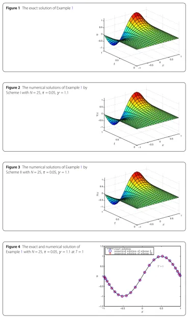
+πt4cosxcos(πx), x∈Λ. The exact solution is

u(x,t) =t4sin(πx).

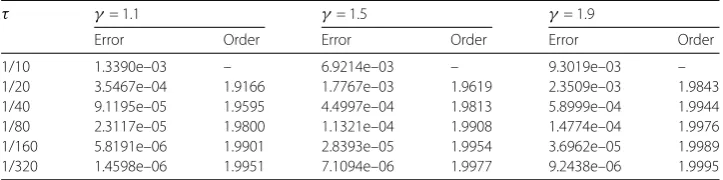
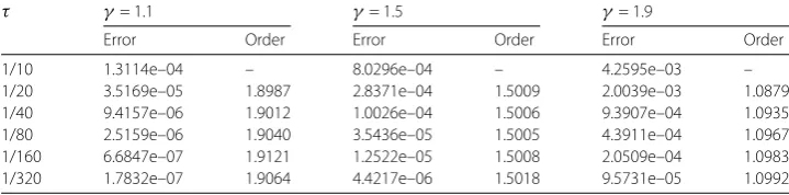
LetN= 25,τ= 0.05, andγ= 1.1. The exact solution of Example1is shown in Fig.1, and numerical solutions by two schemes are shown in Figs.2and3.

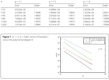
ForT= 1, the exact solution and the numerical solutions of Example1are depicted in Fig.4. From Figs.1–4we can seen that the numerical solutions of two schemes are very similar to the exact solution.

To confirm the temporal accuracy, we chooseNlarge enough such that the space dis-cretization error is negligible compared with the temporal error. Here we takeN= 25 and

Figure 1The exact solution of Example1

Figure 2The numerical solutions of Example1by Scheme I withN= 25,τ= 0.05,γ= 1.1

Figure 3The numerical solutions of Example1by Scheme II withN= 25,τ= 0.05,γ= 1.1

Table 1 H1_{errors and temporal convergence orders of Scheme I for Example1}

τ γ= 1.1 γ= 1.5 γ= 1.9

Error Order Error Order Error Order

1/10 3.5575e–03 – 2.0007e–02 – 9.9520e–02 –

1/20 9.5487e–04 1.8975 7.1177e–03 1.4910 4.6896e–02 1.0855

1/40 2.5607e–04 1.8987 2.5248e–03 1.4953 2.1983e–02 1.0931

1/80 6.8643e–05 1.8994 8.9413e–04 1.4976 1.0280e–02 1.0965

1/160 1.8396e–05 1.8997 3.1638e–04 1.4988 4.8015e–03 1.0983

1/320 4.9297e–06 1.8998 1.1190e–04 1.4994 2.2413e–03 1.0992

Table 2 L2errors and temporal convergence rates of Scheme II for Example1

τ γ= 1.1 γ= 1.5 γ= 1.9

Error Order Error Order Error Order

1/10 1.3390e–03 – 6.9214e–03 – 9.3019e–03 –

1/20 3.5467e–04 1.9166 1.7767e–03 1.9619 2.3509e–03 1.9843

1/40 9.1195e–05 1.9595 4.4997e–04 1.9813 5.8999e–04 1.9944

1/80 2.3117e–05 1.9800 1.1321e–04 1.9908 1.4774e–04 1.9976

1/160 5.8191e–06 1.9901 2.8393e–05 1.9954 3.6962e–05 1.9989

1/320 1.4598e–06 1.9951 7.1094e–06 1.9977 9.2438e–06 1.9995

Figure 5 γ= 1.5,τ= 0.001, errors of Example1

versus the polynomial degreeN

and Table2shows the errorsu(T) –uM

Nand temporal convergence orders of Scheme II,

which are consistent with our theoretical analysis. The convergence order is given by the formula

Order =loge1–loge2

logτ1–logτ2

,

whereeiis the error corresponding toτi,i= 1, 2.

Example2 (Finite regular solution) We consider problem (1)–(3) withp(x) = 2 –sinx,

q(x) = 1 +cosx, and the source term

g(x,t) = 6

Γ(4 –γ)t

3–γ_{(1 –x)(1 +x)}2_x16_{3 +t}3_{(1 +cosx)(1 –x)(1 +x)}2_x16₃

–2 9t

3_{(2 –sinx)104 + 152x– 209x}2_{– 275x}3_x10₃

+t

3

3 cosx

16 + 19x– 22x2– 25x3x133_{, x}∈_Λ.

The exact solution is

u(x,t) =t3(1 –x)(1 +x)2x163_,

which has finite regularity (we can readily to verify thatu∈H5_{(Λ) butu∈/H}6_(Λ)).

For comparison, we depict the exact and numerical solutions at different times T in Fig.6. Here we chooseN= 50,τ = 0.05, andγ = 1.1. The black curve denotes the exact solution, blue “O” represents the numerical solution of Scheme I and red “+” denotes the numerical solution of Scheme II. Different curves with symbols “O” and “+” represent the true solution and numerical solutions at different timeT, respectively. The exact solution and numerical solutions match well at different timesTas shown in Fig.6, which illustrates that two numerical schemes effectively approximate the exact solution.

We takeN= 100, which is large enough such that the space discretization error is negli-gible compared with the temporal error. Table3lists the errorsu(T) –uM

N1and temporal

Figure 6The exact and numerical solutions of Example2withN= 50,τ= 0.05,γ= 1.1

Table 3 H1errors and temporal convergence orders of Scheme I for Example2

τ γ= 1.1 γ= 1.5 γ= 1.9

Error Order Error Order Error Order

1/10 1.3114e–04 – 8.0296e–04 – 4.2595e–03 –

1/20 3.5169e–05 1.8987 2.8371e–04 1.5009 2.0039e–03 1.0879

1/40 9.4157e–06 1.9012 1.0026e–04 1.5006 9.3907e–04 1.0935

1/80 2.5159e–06 1.9040 3.5436e–05 1.5005 4.3911e–04 1.0967

1/160 6.6847e–07 1.9121 1.2522e–05 1.5008 2.0509e–04 1.0983

Table 4 L2_{errors and temporal convergence orders of Scheme II for Example2}

τ γ= 1.1 γ= 1.5 γ= 1.9

Error Order Error Order Error Order

1/10 9.9259e–05 – 4.2089e–04 – 5.3029e–04 –

1/20 2.5339e–05 1.9698 1.0644e–04 1.9834 1.3229e–04 2.0031

1/40 6.4011e–06 1.9850 2.6763e–05 1.9917 3.3056e–05 2.0007

1/80 1.6082e–06 1.9929 6.7107e–06 1.9957 8.2649e–06 1.9998

1/160 4.0289e–07 1.9970 1.6808e–06 1.9973 2.0665e–06 1.9998

1/320 1.0154e–07 1.9884 4.2141e–07 1.9959 5.1665e–07 1.9999

Figure 7 γ= 1.5,τ= 0.001, errors of Example2

versus the polynomial degreeN

convergence orders of Scheme I, and Table4shows the errorsu(T) –uM

Nand temporal

convergence orders of Scheme II for Example2, which are consistent with our theoretical analysis. Here we chooseT= 1.

Now we investigate the spatial accuracy with respect to the polynomial degreeN. We fix the time stepτ= 0.001 to avoid the contamination of the temporal error and illustrate the caseγ = 1.5.

In Fig.7, we present the errors with respect to the polynomial degreeN in a log-log scale for Example2. Since its exact solution belongs toH5(Λ), but not toH6(Λ), we can see from Fig.7that the convergence rate is betweenN–4_andN–5_{, which conforms with}

our theoretical analysis.

6 Conclusions

In this paper, we presented and analyzed two fully discrete spectral schemes for the frac-tional diffusion-wave equation with variable coefficients in a bounded domain, one based on its original form and the other based on its equivalent fractional integro-differential form. The stability and convergence of two schemes were rigorously established. We car-ried out some numerical experiments to support the theoretical results. From numerical examples we can seen that two numerical schemes work well on time-fractional diffusion-wave equations, no matter the solution is sufficiently smooth or of finite regularity. The schemes presented in the paper can also be extended to solve two- or three-dimensional time fractional diffusion-wave equations on rectangular or cubical domains.

Funding

Competing interests

The authors declare that they have no competing interests.

Authors’ contributions

All authors read and approved the final manuscript.

Author details

1_{School of Mathematics & Computing Science, Guilin University of Electronic Technology, Guilin, China.}2_{School of}

Mathematics & Systems Science & LMIB, Beihang University, Beijing, China. 3_{Beijing Computational Science Research}

Center, Beijing, China.

Publisher’s Note

Springer Nature remains neutral with regard to jurisdictional claims in published maps and institutional affiliations.

Received: 30 November 2018 Accepted: 21 September 2019 References

1. Ross, B.: A brief history and exposition of the fundamental theory of fractional calculus. In: Ross, B. (ed.) Fractional Calculus and Its Applications, pp. 1–36. Springer, Berlin (1975)

2. Glöckle, W.G., Nonnenmacher, T.F.: A fractional calculus approach to self-similar protein dynamics. Biophys. J.68, 46–53 (1995)

3. Kutner, R.: Coherent spatio-temporal coupling in fractional wanderings, renewed approach to continuous-time Lévy flights. In: Pe¸kalski, A., Sznajd-Weron, K. (eds.) Anomalous Diffusion: From Basics to Applications, pp. 1–14. Springer, Berlin (1999)

4. Metzler, R., Klafter, J.: The random walk’s guide to anomalous diffusion: a fractional dynamics approach. Phys. Rep.

339, 1–77 (2000)

5. Scalas, E., Gorenflo, R., Mainardi, F.: Fractional calculus and continuous-time finance. Physica A284, 376–384 (2000) 6. Magin, R.L.: Fractional Calculus in Bioengineering. Begell House Publishers Inc., Redding (2006)

7. Cuesta, E.: Some advances on image processing by means of fractional calculus. In: Machado, J.A.T., Luo, A.C.J., Barbosa, R.S., Silva, M.F., Figueiredo, L.B. (eds.) Nonlinear Science and Complexity, pp. 265–271. Springer, Dordrecht (2011)

8. Machado, J.T., Kiryakova, V., Mainardi, F.: Recent history of fractional calculus. Commun. Nonlinear Sci. Numer. Simul.

16, 1140–1153 (2011)

9. Baleanu, D., Agarwal, P.: Certain inequalities involving the fractionalq-integral operators. Abstr. Appl. Anal.2014, Article ID 371274 (2014)

10. Kıymaza, ˙I.O., Çetinkaya, A., Agarwal, P.: An extension of Caputo fractional derivative operator and its applications. J. Nonlinear Sci. Appl.9, 3611–3621 (2016)

11. Agarwal, P., Jain, S., Mansour, T.: Further extended Caputo fractional derivative operator and its applications. Russ. J. Math. Phys.24, 415–425 (2017)

12. Agarwal, P.: Fractional integration of the product of two H-functions and a general class of polynomials. In: Anastassiou, G.A., Duman, O. (eds.) Advances in Applied Mathematics and Approximation Theory, pp. 359–374. Springer, Berlin (2013)

13. Choi, J., Agarwal, P.: Certain integral transform and fractional integral formulas for the generalized Gauss hypergeometric functions. Abstr. Appl. Anal.2014, Article ID 735946 (2014)

14. Stynes, M., Gracia, J.L.: A finite difference method for a two-point boundary value problem with a Caputo fractional derivative. IMA J. Numer. Anal.35, 698–721 (2015)

15. Meerschaert, M., Tadjeran, C.: Finite difference approximations for fractional advection dispersion flow equations. J. Comput. Appl. Math.172, 65–67 (2004)

16. Alikhanov, A.A.: A new difference scheme for the time fractional diffusion equation. J. Comput. Phys.280, 424–438 (2015)

17. Alikhanov, A.A.: Stability and convergence of difference schemes approximating a two-parameter nonlocal boundary value problem for time-fractional diffusion equation. Comput. Math. Model.26, 252–272 (2015)

18. Ervin, V.J., Heuer, N., Roop, J.P.: Numerical approximation of a time dependent, nonlinear, space-fractional diffusion equation. SIAM J. Numer. Anal.45, 572–591 (2007)

19. Deng, W.H.: Finite element method for the space and time fractional Fokker–Planck equation. SIAM J. Numer. Anal.

47, 204–226 (2008)

20. Zhang, H.M., Liu, F.W., Anh, V.: Galerkin finite element approximation of symmetric space-fractional partial differential equations. Appl. Math. Comput.217, 2534–2545 (2010)

21. Mustapha, K., McLean, W.: Superconvergence of a discontinuous Galerkin method for fractional diffusion and wave equations. SIAM J. Numer. Anal.51, 491–515 (2013)

22. Xu, Q.W., Hesthaven, J.S.: Discontinuous Galerkin method for fractional convection–diffusion equations. SIAM J. Numer. Anal.52, 405–423 (2014)

23. Zayernouri, M., Karniadakis, G.E.: Fractional spectral collocation method. SIAM J. Sci. Comput.36, A40–A62 (2014) 24. Chen, F., Xu, Q.W., Hesthaven, J.S.: A multi-domain spectral method for time-fractional differential equations.

J. Comput. Phys.293, 157–172 (2015)

25. Bhrawy, A.H., Baleanu, D., Mallawi, F.: A new numerical technique for solving fractional sub-diffusion and reaction sub-diffusion equations with a non-linear source term. Therm. Sci.19, S25–S34 (2015)

26. Bhrawy, A.H., Zaky, M.A., Baleanu, D.: New numerical approximations for space-time fractional Burgers’ equations via a Legendre spectral-collocation method. Rom. Rep. Phys.67, 340–349 (2015)

28. Doha, E.H., Abdelkawy, M.A., Amin, A.Z.M., Baleanu, D.: Spectral technique for solving variable-order fractional Volterra integro-differential equations. Numer. Methods Partial Differ. Equ.34, 1659–1677 (2017)

29. Povstenko, Y.: Linear Fractional Diffusion-Wave Equation for Scientists and Engineers. Springer, Cham (2015) 30. Schneider, W.R., Wyss, W.: Fractional diffusion and wave equations. J. Math. Phys.30, 134–144 (1989)

31. Agrawal, O.P.: Solution for a fractional diffusion-wave equation defined in a bounded domain. Nonlinear Dyn.29, 145–155 (2002)

32. Pskhu, A.V.: The fundamental solution of a diffusion-wave equation of fractional order. Izv. Math.73, 351–392 (2009) 33. Chen, J., Liu, F., Anh, V., Shen, S., Liu, Q., Liao, C.: The analytical solution and numerical solution of the fractional

diffusion-wave equation with damping. Appl. Math. Comput.219, 1737–1748 (2012)

34. Sun, Z.Z., Wu, X.N.: A fully discrete difference scheme for a diffusion-wave system. Appl. Numer. Math.56, 193–209 (2006)

35. Huang, J., Tang, Y., Vázquez, L., Yang, J.: Two finite difference schemes for time fractional diffusion-wave equation. Numer. Algorithms64, 707–720 (2013)

36. Wang, Z.B., Vong, S.: Compact difference schemes for the modified anomalous fractional sub-diffusion equation and the fractional diffusion-wave equation. J. Comput. Phys.277, 1–15 (2014)

37. Wang, Y.M.: A compact finite difference method for a class of time fractional convection–diffusion-wave equations with variable coefficients. Numer. Algorithms70, 625–651 (2015)

38. Diethelm, K.: The Analysis of Fractional Differential Equations: An Application-Oriented Exposition Using Differential Operators of Caputo Type. Springer, Berlin (2010)

39. Podlubny, I.: Fractional Differential Equations. Academic Press, San Diego (1999)

40. Canuto, C., Hussaini, M.Y., Quarteroni, A., Zang, T.A.: Spectral Methods: Fundamentals in Single Domains. Springer, Berlin (2006)

41. Sun, Z.Z.: The Method of Order Reduction and Its Application to the Numerical Solutions of Partial Differential Equations. Science Press, Beijing (2009)

42. Tian, W., Zhou, Z., Deng, W.: A class of second order difference approximations for solving space fractional diffusion equations. Math. Comput.84, 1703–1727 (2015)

43. Heywood, J.G., Rannacher, R.: Finite-element approximation of the nonstationary Navier–Stokes problem. Part IV: error analysis for second-order time discretization. SIAM J. Numer. Anal.27, 353–384 (1999)

44. Chen, H., Lü, S.J., Chen, W.P.: A unified numerical scheme for the multi-term time fractional diffusion and diffusion-wave equations with variable coefficients. J. Comput. Appl. Math.330, 380–397 (2018)