Integrated gradient interpretation techniques for 2D and 3D
gravity data interpretation
Hakim Saibi1, Jun Nishijima1, Sachio Ehara1, and Essam Aboud2
1Department of Earth Resources Engineering, Kyushu University, Fukuoka 812-8581, Japan 2National Research Institute of Astronomy and Geophysics, P.O. Box 227, 11722 Helwan, Cairo, Egypt (Received September 29, 2005; Revised February 28, 2006; Accepted February 28, 2006; Online published July 26, 2006)
The Obama geothermal field is located on the western part of Kyushu Island, Japan. This area has importance due to its high geothermal content which attracts sporadic researchers for study. In 2003 and 2004, Obama was covered by gravity surveys to monitor and evaluate the geothermal field. In this paper, the surveyed gravity data will be used in order to delineate and model the subsurface structure of the study area. Gradient methods such as analytic signal and vertical derivatives were applied to the gravity data. The available borehole data and the results of the gradient interpretation techniques were used to model the Obama geothermal field. In general, the obtained results show that the gradient interpretation techniques are useful to obtain geologic information from gravity data.
Key words:Analytic Signal, gravity interpretation, Obama geothermal area.
1.
Introduction
The Obama geothermal field is located on the western part of Kyushu Island, southwestern Japan (Fig. 1), on the western foot of Unzen volcano and in front of Chijiwa Bay. The Obama geothermal area is one of the most promising geothermal fields in Japan, and therefore study of its struc-ture contributes to a potentially useful understanding of its reservoir characteristics.
In order to delineate the subsurface structure of the Obama area, gradient techniques were applied to the grav-ity data of the study area. In the early 1970’s, a variety of automatic and semiautomatic methods, based on the use of gradients of the potential field, were developed as efficient tools for the determination of geometric parameters, such as locations of boundaries and depth of the causative sources (e.g. O’Brien, 1972; Nabighian, 1972, 1974; Cordell, 1979; Murthy, 1985; Barongo, 1985; Blakely and Simpson, 1986; Hansenet al., 1987; Hansen and Simmonds, 1993; Reidet al., 1990; Keating and Pilkington, 1990; Ofoegbu and Mo-han, 1990; Roestet al., 1992; Marcotteet al., 1992; Mar-son and Klingele, 1993; Hsuet al., 1996, 1998; Salem and Ravat, 2003; Keating and Pilkington, 2004; Aboudet al., 2005). The success of these methods results from the fact that quantitative or semi-quantitative solutions are found with no or few assumptions.
In this work, gravity data of the Obama geothermal field was analyzed and interpreted using the analytic signal and vertical derivative methods. Initially, because the Obama area is covered by reclaimed land that enlarges the noise, the upward continuation technique was used as a noise-filter to reduce the noise. Then, an analytic signal was applied to the
Copyright cThe Society of Geomagnetism and Earth, Planetary and Space Sci-ences (SGEPSS); The Seismological Society of Japan; The Volcanological Society of Japan; The Geodetic Society of Japan; The Japanese Society for Planetary Sci-ences; TERRAPUB.
gravity data in order to delineate the borders/contacts of the geologic boundaries. Once the analytic signal is applied, the depths to these boundaries were estimated using the Nabighian method (1972). In order to calculate the second vertical derivative of the gravity data, Fast Fourier Trans-form (FFT) was applied to the gravity data. Finally, the results of the analytic signal, depth estimation, and second vertical derivative techniques were used to create a geologic model expressing the subsurface structure of the Obama area.
Geologically, the Obama area is composed of
Quaternary-Neogene volcanic formations. The
base-ment rock is composed of Pliocene (Neogene) formations and the overlying sedimentary rock is composed essentially
of Quaternary formations (Fig. 2). Previous geological
studies indicated the existence of faults striking mainly E-W (New Energy Developing Organization, 1988; Saibi
et al., 2006). However, a N-S trend can be observed in the area, namely the Obama fault bordering the western coast of the Obama area ( ¯Ota, 1973; Saibiet al., 2006).
1.1 Gravity data
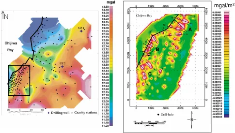
The Obama geothermal field was covered by gravity sur-veys as a routine method for monitoring and evaluating the geothermal reservoir. The gravity data collected during 2003 and 2004 were used in this study in an attempt to de-lineate the subsurface structure of the Obama area. This will hopefully lead to exploration of new features that can help in maximizing the production and minimizing the cost of energy production. A density of 2.3 g/cm3 (Murata, 1993) was used to produce the Bouguer anomaly map of the study area (Fig. 3).
Gravity was surveyed over an area of 4 km2. Surveys of the GPS (Topcon GP-SX1) single frequency type were con-ducted using the kinematic method, which can be placed anywhere in radio contact of the base station to measure
Fig. 1. Location map of Obama geothermal area, Japan.
cations precise to the centimeter level, and the Scintrex CG-3M gravimeter, a very sensitive mechanical balance which detects changes in the gravitational field to one part in a mil-lion. The gravity data was corrected for temporal variations (drift and tides). The ocean loads and tides were calculated
using the computer program GOTIC2 (Matsumoto et al.,
2001). The coordinates of stations and their altitudes were measured by GPS, with an error of±10 cm in altitude, and approximately±0.03 mgal of error in Bouguer gravity. The terrain correction was applied for the observed gravity us-ing the computer program KS-110-1 (Katsuraet al., 1987) with a mesh of 250 m.
Visual inspection of Fig. 3 shows that the area is charac-terized by positive gravity values covering the whole area, ranging between 11.2 and 13.5 mgal, and increasing in the eastern and southern parts of the map area. This could be related to the low gradient in the subsurface structure. The depth to the basement from drill-hole data is 500 m (New Energy Developing Organization, 1988). The ob-served variations in the anomalies reflect the half graben structure associated with the volcano-tectonic depression zone of Shimabara peninsula.
2.
Applications and Results
2.1 Analytic signal methodThe basic concepts of the analytic signal method in 2D for magnetic data were extensively discussed by Nabighian (1972, 1974 and 1984) and Green and Stanley (1975). Their counterparts, in the case of gravity data, have been in-troduced by Klingele et al.(1991). Marson and Klingele (1993) define the analytic signal of the vertical gravity gra-dient produced by a 3D source as follows:
Ag(x,y)=
∂
g
∂x
2
+
∂g
∂y
2
+
∂g
∂z
2
, (1)
Fig. 2. Geologic map of Obama geothermal area modified by the New Energy Developing Organization (1988). The black rectangle indicates the study area and the red rectangle indicates the southern part of the study area.
where|Ag(x,y)|is the amplitude of the analytic signal at
(x,y),gis the observed gravity field at(x,y), and (∂∂gx,∂∂gy, and∂∂gz) are the two horizontal and vertical derivatives of the gravity field, respectively. The other unusual feature of our technique is the use of the analytic signal for gravity data. Straightforward application of the Poisson relation (Pois-son, 1826; Baranov, 1957) and correspondence between gravity and magnetic fields for homogeneous bodies would suggest use of the analytic signal of the vertical gradient of gravity data. This relates the vertical gradient of gravity data from a given source to the magnetic effect of the same source. Starting from this consideration, one can apply magnetic interpretation methods to gravity data. Klingele
13.50 black rectangle indicates the southern part of the study area. The black line indicates the coastline.
of the Bouguer anomalies into vertical gradient anomalies. Stanley and Green (1976) stated that gravity gradient infor-mation is more sensitive to geological structure than grav-ity itself, and gradient interpretation is less susceptible to interference from neighbouring structures. The application of the analytic signal method to gravity data was first sug-gested by Nabighian (1972), but he did not apply this con-cept to gravity data. Hansenet al.(1987) suggested that the straightforward application of Poisson’s relation could lead to the use of the analytic signal method for gravity data. For geologic models, the shape of the analytic signal is a bell-shaped symmetric function located above the source body. The analytic signal maxima occur directly over the edges of source bodies. The analytic signal is peaked over the lo-cation of the top of the contact. In addition, depths can be obtained from the shape of the analytic signal (MacLeodet al., 1993). The analytic signal method, also known as the total gradient method, as defined here, produces a particular type of calculated gravity anomaly enhancement map used for defining, in a map sense, the edges (boundaries) of ge-ologically anomalous density distributions. Mapped max-ima (ridges and peaks) in the calculated analytic signal of a gravity anomaly map locate the anomalous source body edges and corners (e.g., basement fault block boundaries, basement lithology contacts, fault/shear zones, igneous and salt diapirs, etc.). Analytic signal maxima have the useful property that they occur directly over faults and contacts, regardless of the structural dip present.
2.2 Depth estimation
The analytic signal anomaly over a 2-D magnetic contact located atx and at depthh is described by the expression
1
Fig. 4. Analytic signal of the first vertical gradient of the Bouguer gravity map of the southern part of the Obama area. Lines 1–19 are the selected profiles that were used to estimate the depths from the analytic signal. The black line indicates the coastline.
0 10 20 30 40 50 60 70
Fig. 5. Amplitude of the analytic signal of profile 1 of the study area.
(after Nabighian, 1972):
|A(x)| =α 1
h2+x21/2, (2) where|A(x)|is the analytic signal andαis the amplitude factor. For a contact, taking the second derivative of Eq. (2) with respect tox produces the following (MacLeodet al., 1993): After rearranging Eq. (3), we obtain (MacLeodet al., 1993):
xi = √
Table 1. Estimated depths from analytic signal method at the contacts.
Profile Depth m. Profile Depth m. Profile Depth m. Profile Depth m. Profile Depth m.
Profile 1 39 Profile 5 42 Profile 9 29 Profile13 42 Profile17 50
Profile 2 39 Profile 6 42 Profile10 32 Profile14 39 Profile18 25
Profile 3 46 Profile 7 46 Profile 11 35 Profile15 64 Profile19 42
Profile 4 33 Profile 8 46 Profile12 42 Profile16 42
A
B
C
0.00053 0.00048 0.00043 0.00038 0.00035 0.00032 0.00029 0.00026 0.00023 0.00021 0.00019 0.00017 0.00014 0.00013 0.00011 0.00009 0.00007 0.00005 0.00003 0.00001 -0.00001 -0.00003 -0.00005 -0.00007 -0.00009 -0.00011 -0.00013 -0.00015 -0.00017 -0.00020 -0.00022 -0.00024 -0.00027 -0.00030 -0.00033 -0.00037 -0.00041 -0.00045 -0.00052 -0.00061
mgal/m
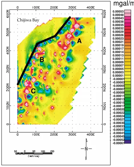
2Fig. 6. Second vertical derivative map of the Bouguer gravity data of the southern part of the Obama field. The black line indicates the coastline.
wherehis the depth to the top of contact andxiis the width
of the anomaly between inflection points.
2.3 Results of analytic signal method
The analytic signal signature of the southern part of the Obama field was calculated (Fig. 4) from the first vertical gradient of the Bouguer gravity data, in the frequency do-main using the Fast Fourier Transform technique (Blakely, 1995). Higher values of the analytic signal are observed at three regions labeled A, B, and C as shown in Fig. 4, which indicate that these regions have significant density contrasts that produce identifiable signatures on the map. To estimate the depth to the contacts from the analytic signal, 19 pro-files were selected over the regions A, B, and C in which contrasts could be found. Equation (4) was used to calcu-late the depth for each profile at the top of contacts. Table 1 shows the depth values. Generally, the depth values for re-gion (A) have an average value of 44.4 m, for rere-gion (B) an average of 42 m, and for region (C) an average of 39 m. The calculated depths from the Euler deconvolution method (Saibiet al., 2005) ranged between 50 and 100 m. We can observe coherent results between the Euler method and the
0 m.
30 m.
80 m.
110 m.
RECLAIMED LAND
TUFF BRECCIA
ANDESITIC LAVA
density = 2.2 g/cm
density = 2.4 g/cm 3
3
Fig. 7. Stratigraphic log of drill-hole at the southern part of the Obama area.
analytic signal method. To test the usefulness of the ana-lytic signal in the gravity case, we have calculated the depth to the contact from profile 1 (Fig. 5), where a drill-hole was drilled recently. The drill-hole data shows that a main frac-tured zone is situated between 110 and 121 m depth. On the other hand, the drill-hole data gives information that in-dicates the existence of a zone of clay minerals at 45 m depth. Generally, a clay mineral zone indicates a leaching-weathering phenomenon, or simple alteration caused by in-trusion of water, which means the existence of lateral flow reaching the top of contacts. Drilling report results agree with the analytic signal results (42 m depth).
2.4 Second vertical derivative (SVD)
Line 1
Line 2
Line 3 Line 4
Line 5
Line 6
A
B
C
0.229 0.209 0.189 0.173 0.160 0.150 0.139 0.128 0.119 0.111 0.103 0.094 0.088 0.080 0.072 0.054 0.057 0.051 0.044 0.038 0.029 0.022 0.016 0.008 0.001 -0.007 -0.013 -0.022 -0.030 -0.039 -0.046 -0.056 -0.066 -0.077 -0.087 -0.101 -0.118 -0.136 -0.158 -0.192
mgal
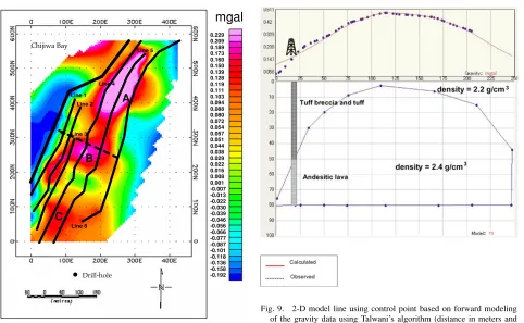
Fig. 8. Enhanced Bouguer gravity map using separation filter of the southern part of the Obama area. The black line indicates the coastline.
to the “curvature” of the input gravity (Fig. 6). The SVD map tends to emphasize local anomalies and isolate them from the regional background. The SVD enhances near-surface effects at the expense of deeper anomalies. The quantity 0 mgal/m2 should indicate the edges of local ge-ological features. Three regions can be seen: A, B, and C, with almost the same positions determined by the analytic signal method. Unfortunately, SVD amplifies noise and so is capable of producing many second derivative anomalies that could be artificial.
2.5 2D forward modeling of enhanced bouguer
The southern part of the Obama area is covered by re-claimed land about 30 m in thickness (Fig. 7). Upward Continuation (UC) filtering was carried out on the grav-ity data to remove the effect of the reclaimed land. The UC serves to smooth out near-surface effects (shorter— wavelength anomalies) after calculating the gravity field at an elevation higher than that at which the gravity field is measured. The Enhanced Bouguer (Fig. 8) may remove the trend caused by the reclaimed land. The Enhanced Bouguer gravity data was calculated using this expression:
BouguerEnhanced=Bouguerwithout transformation
−BouguerContinued upward 50 m. (5)
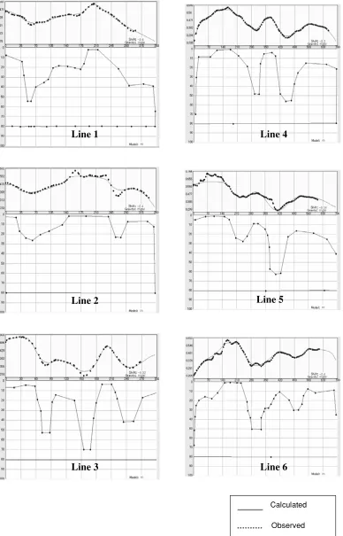
After calculating the Enhanced Bouguer gravity, six par-allel lines were selected in order to get a geologic model of the shallow layers in the southern part of Obama. The Enhanced Bouguer was forward modeled using the algo-rithm of Talwaniet al.(1959) and a contrast density of−0.2 g/cm3. Figure 9 shows a 2D model with the control point
Fig. 9. 2-D model line using control point based on forward modeling of the gravity data using Talwani’s algorithm (distance in meters and gravity in mGal).
(drill-hole) using Talwani’s algorithm and shows the true depth value of the tuff breccia layer in relation to other lines, which will be taken into consideration for forward model-ing of lines 1–6 (Figs. 10 and 11).
3.
Discussion
The total area of the southern part of the Obama field is around 240 m2. The gradient interpretation techniques can-not detect deep anomalies. All these methods use deriva-tives of the first and second order; this may add noise to the field and affect the results. Here, we applied many transformations in order to minimize the noise and enhance the gravity data. The analytic signal method defines the edges of geologically anomalous density distributions and the maxima in the calculated analytic signal of a gravity anomaly map to locate the anomalous source body edges and corners; in our case are andesitic lava bodies. The ig-neous rocks are bordered by normal faults which contain drained water (trace of alteration zones). To estimate the depth from the analytic signal, we have used the method of MacLeod et al.(1993) who stated that the contact model will underestimate the depth by 18%, especially in residual data, as in this case. Our results show noise ranging from 15 to 18%, taking all noise-source possibilities into account. Figure 12 shows the geologic model of the southern part of the Obama field integrated from gradient interpretation techniques of gravity data.
4.
Conclusions
grav-Line 1
Line 2
Line 3
Line 4
Line 6
Calculated
Observed
Line 5
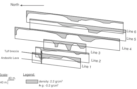
Fig. 10. 2-D conceptual structural model (line 1–line 6) based on forward modeling of the gravity data.
ity field. The depths to the contacts vary between 39 and 64 m. All the methods show three bodies A, B, and C elon-gated north-east to south-west. The bodies represent the up-doming of andesitic lava. This structure is a typical graben related to the regional geology. The study area is
Line 1
40 m. density: 2.2 g/cm
g: -0.2 g/cm
Scale: Legend:
3 3
Fig. 11. 3-D view of 2-D gravity forward modeling of lines 1–6 of the southern part of Obama.
BODY A BODY B BODY C
Trend of fault NE-SW
40 m depth
Alterated zone
0 m 700 m
Fig. 12. Schematic geologic model of a north-east cross-section at the southern part of the Obama area.
Acknowledgments. The first author would like to thank Prof. Richard Hansen (School of Mines, Colorado) for his suggestions and comments. We also thank two anonymous reviewers for their revisions and useful comments which improved the paper. We would like to thank Ms. Katie Kovac (Energy and Geoscience In-stitute, USA) for suggesting a number of improvements in this manuscript. We gratefully acknowledge the financial support of the Ministry of Education, Culture, Science and Technology, Gov-ernment of Japan in the form of a Scholarship.
References
Aboud, E., A. Salem, and K. Ushijima, Subsurface structural mapping of Gabel El-Zeit area, Gulf of Suez, Egypt using aeromagnetic data,Earth Planets Space,57, 755–760, 2005.
Baranov, V., A new method for interpretation of aeromagnetic maps: pseudo-gravimetric anomalies,Geophysics,22, 359–383, 1957. Barongo, J. O., Method for depth estimation on aeromagnetic vertical
gradient anomalies,Geophysics,50(6), 963–968, 1985.
Blakely, R. J.,Potential Theory in Gravity and Magnetic Applications, Cambridge University Press, 1995.
Blakely, R. J. and R. W. Simpson, Approximating edges of source bodies from magnetic or gravity anomalies,Geophysics (short note),51(7), 1494–1498, 1986.
Cordell, L., Gravimetric expression of graben faulting in Santa Fe Coun-try and the Espanola Basin, New Mexico, inGuidebook to Santa Fe Country, 30th Field Conference, edited by R. V. Ingersoll, New Mexico Geological Society, pp. 59–64, 1979.
Green, R. and J. M. Stanley, Application of a Hilbert transform method to the interpretation of surface-vehicle magnetic data, Geophysical Prospecting,23, 18–27, 1975.
Hansen, R. O. and M. Simmonds, Multiple-source Werner deconvolution,
Geophysics,58(12), 1792–1800, 1993.
Hansen, R. O., R. S. Pawlowski, and X. Wang, Joint use of analytic sig-nal and amplitude of horizontal gradient maxima for three-dimensiosig-nal gravity data interpretation, 57th SEG meeting, New Orleans, extended Abstracts, pp. 100–102, 1987.
Hsu, S. K., D. Coppens, and C. T. Shyu, Depth to magnetic source using
the generalized analytic signal,Geophysics,63, 1947–1957, 1998. Hsu, S. K., J. C. Sibuet, and C. T. Shyu, High-resolution detection of
geologic boundaries from potential anomalies: an enhanced analytic signal technique,Geophysics,61, 373–386, 1996.
Katsura, I., J. Nishida, and S. Nishimura, A computer program for terrain correction of gravity using KS-110-1 topographic data,Butsuri-Tansa, 40(3), 161–175, 1987 (in Japanese with Abstract in English). Keating, P. B. and M. Pilkington, An automated method for the
interpre-tation of magnetic vertical-gradient anomalies,Geophysics,55(3), 336– 343, 1990.
Keating, P. and M. Pilkington, Euler deconvolution of the analytic signal and its application to magnetic interpretation,Geophysical Prospecting, 52, 165–182, 2004.
Klingele, E. E., I. Marson, and H. G. Kahle, Automatic interpretation of gravity gradiometric data in two dimensions: vertical gradient, Geo-physical Prospecting,39, 407–434, 1991.
MacLeod, I. N., K. Jones, and T. F. Dai, 3-D analytic signal in the interpre-tation of total magnetic field data at low magnetic latitudes,Exploration Geophysics, 679–688, 1993.
Marcotte, D. L., C. D. Hardwick, and J. B. Nelson, Automated interpre-tation of horizontal magnetic gradient profile data,Geophysics,57(2), 288–295, 1992.
Marson, I. and E. E. Klingele, Advantages of using the vertical gradient of gravity for 3-D interpretation,Geophysics,58(11), 1588–1595, 1993. Matsumoto, K., T. Sato, T. Takanezawa, and M. Ooe, GOTIC2: A program
for computation of ocean tidal loading effect,J. Geod. Soc. Japan,47, 243–248, 2001.
Murata, Y., Estimation of optimum average surficial density from gravity data: An objective Bayesian approach,J. Geophys. Res.,98(B7), 12097– 12109, 1993.
Murthy, I. V. R., The midpoint method: Magnetic interpretation of dykes and faults,Geophysics,50(5), 834–839, 1985.
Nabighian, M. N., The analytic signal of two-dimensional magnetic bod-ies with polygonal cross-section: its propertbod-ies and use for automated anomaly interpretation,Geophysics,37(3), 507–517, 1972.
Nabighian, M. N., Additional comments on the analytic signal of two-dimensional magnetic bodies with polygonal cross-section,Geophysics, 39(1), 85–92, 1974.
Nabighian, M. N., Toward a three-dimensional automatic interpretation of potential field data via generalized Hilbert transforms: Fundamental relations,Geophysics,49(6), 780–786, 1984.
New Energy Developing Organization, Geothermal development research document, Unzen Western Region,New Energy Developing Organiza-tion, No. 15, 1988.
O’Brien, D. P., CompuDepth—a new method for depth-to-basement cal-culation, presented at the 42nd Meeting of the Society of Exploration Geophysicists, Anaheim, CA, 1972.
Ofoegbu, C. O. and N. L. Mohan, Interpretation of aeromagnetic anoma-lies over part of southeastern Nigeria using three-dimensional Hilbert transformation,Pageoph,134, 13–29, 1990.
¯
Ota, K., A study of hot springs on the Shimabara peninsula,The science reports of the Shimabara volcano observatory, the Faculty of Science, Kyushu University, No. 8, pp. 1–33, 1973.
Poisson, S. D., M´emoire sur la th´eorie du magn´etisme, M´emoires de l’Acad´emie Royale des Sciences de l’Institut de France, pp. 247–348, 1826 (in French).
Reid, A. B., J. M. Allsop, H. Granser, A. J. Millet, and W. Somerton, Magnetic interpretation in three dimensions using Euler deconvolution,
Geophysics,55(1), 80–91, 1990.
Roest, W. R., J. Verhoef, and M. Pilkington, Magnetic interpretation using the 3-D analytic signal,Geophysics,57(1), 116–125, 1992.
Saibi, H., J. Nishijima, E. Aboud, and S. Ehara, Euler deconvolution of gravity data in geothermal reconnaissance; the Obama geothermal area, Japan,Journal of Exploration Geophysics of Japan, 2006 (in press). Salem, A. and D. Ravat, A combined analytic signal and Euler method
(AN-EUL) for automatic interpretation of magnetic data,Geophysics, 68(6), 1952–1961, 2003.
Stanley, J. M. and R. Green Gravity gradients and the interpretation of the truncated plate,Geophysics,41, 1370–1376, 1976.
Talwani, M., J. L. Worzel, and M. Landisman, Rapid gravity computations for two-dimensional bodies with applications to the Mendocino subma-rine fracture zone,J. Geophys. Res.,64, 49–59, 1959.