Multi layer topology control for long term wireless sensor networks

R E S E A R C H

Open Access

Multi-layer topology control for long-term

wireless sensor networks

Ikjune Yoon

, Dong Kun Noh

and Heonshik Shin

Abstract

Due to the inefficiency of a flat topology, most wireless sensor networks (WSNs) have a cluster or tree structure; but this causes an imbalance of residual energy between nodes, which gets worse over time as nodes become defunct and replacements are inserted. Multiple layers are better then the typical two-layer cluster-based topology, because it can better accommodate nodes with different levels of residual energy. We propose that each node should periodically determine its own layer, as its situation and the network topology changes. We introduce a topology control scheme for long-term WSNs with these features. Simulations show that this scheme can balance node energy levels, and thus extend network lifetime.

Keywords:hierarchical topology, network lifetime, wireless sensor network, topology control, energy adaptive rout-ing, long-term WSN

1 Introduction

Simple wireless sensor networks (WSNs) usually have a flat topology and transmit data using a flooding scheme, of which there are several variants. However, flooding can cause the broadcast storming problem [1], reducing the efficiency and reliability of the WSN.

Hierarchical topology control (TC) schemes [2-5] are designed to overcome the broadcast storming problem and to support in-network processing, which improves network performance. A drawback of hierarchical TC schemes is that an imbalance in residual energy between aggregation nodes and general nodes can occur over time, since the aggregation nodes can be expected to consume energy faster than the others [6]. It is even possible for some aggregation nodes to cease participa-tion in the network because they lack energy. In pre-vious schemes [2,4,7], this problem has been overcome by getting nearby energy-rich nodes to take over the roles of defunct aggregation nodes; or new aggregation nodes must be deployed to extend the lifetime of the WSN.

In a WSN which uses hierarchical TC and operates for a long period, the imbalance in residual energy between the nodes can become serious as the number

of failed and insertions or removals replacement nodes recounts of [8]. Draconian changes to the network topology are also likely to be necessary over time.

We propose new TC scheme designed specially for WSNs which are to be maintained for a long period. It minimizes the variation in residual energy between nodes, and thus extends the network lifetime. This goal is achieved by replacing the usual one- or two-layered topology with multiple layers, which can accommodate a wide range of node energy levels more precisely. This new scheme also gets nodes to change roles dynamically as the energy and traffic context changes. This is neces-sary because the energy level of each node and the net-work topology can both change radically in long-term WSNs. In our scheme, each node periodically deter-mines its own layer in response to its energy status, with traffic and topology information. There has been a lot of research on hierarchical topologies for WSNs; but, to the best of our knowledge, this is the first context-aware multi-layer TC scheme for long-term WSNs.

The rest of this article is organized as follows: We explain the outline of the hierarchical TC and its pro-blems in the next section. In Section 3 we describe our layer-based TC scheme for long-term WSNs. We then evaluate the performance of our algorithm in Section 4 and draw conclusions in Section 5.

* Correspondence: [email protected]

2_{School of Electronic Engineering, Soongsil University, Seoul, Korea}

Full list of author information is available at the end of the article

2 Background 2.1 Preliminaries

Hierarchical TC schemes have been shown to produce considerable savings in the total energy consumption of a WSN because of data aggregation [7]. In a hierarchical TC scheme, the nodes are clustered and a head node is assigned to each cluster. A head node is the leader of its group, with the primary responsibility of collection and aggregation of data from its cluster, and transmission of the aggregated data to the sink. Data aggregation greatly reduces energy consumption, because it reduces the total number of messages to be sent to sink, and hence extends network life time. Clustering involves a config-uration and maintenance overhead; but in practice it has been demonstrated that clustering improves both energy consumption and performance in large WSNs.

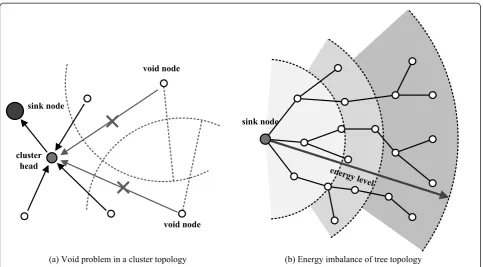
Clustering is not without its problems: a node that cannot act as a cluster head and is not near to a cluster head becomes void, as shown in Figure 1a; and the clus-ter heads consume much more energy than the other nodes, leading to an imbalance across the network. This effect also occurs in a tree-based hierarchical topology, as nodes near the sink node have to transmit consider-ably more data than those at the rim of the network [9], as shown in Figure 1b.

2.2 Related work

Oyman and Ersoy [8] investigated the choice of multiple sinks. They use a cluster scheme in which the sinks act

as cluster-heads, and each node only reports to one cluster-head. Das and Dutta [10] proposed a similar method of sink selection, designed to minimize overall energy consumption.

Buratti et al. [11-13] considered the reachability of multiple sinks in tree-based topologies with fixed node and sink densities.

Kim and Lee [14], and Fan et al. [15] used a spanning tree to control a topology in multi-sink WSNs. Kim and

Lee’s scheme reconfigures itself automatically when

nodes fail, increasing network lifetime.

Fan et al. [15] proposed a three-layer topology for large-scale WSNs in which each layer has its own role. They provide an algorithm that finds all the bottleneck nodes and eliminates them.

Ciciriello et al. [16] introduced a scheme in which the search for a sink topology is mapped to a multi-commodity network design problem. This scheme peri-odically adapts message paths to reduce the number of network links that are used, increasing the efficiency of data transmission.

Intanagonwiwat et al. [17] create a tree which is lim-ited to a single sink at its root. Paths from sensor nodes nearer to the sink are added earlier gradually.

Other authors [18-20] have also utilized a three-layer topology as the basis for control algorithms for static WSNs. Sharma et al. [18] create high-performance clus-ters and zonal sink nodes in order to increase the life-time of sensor nodes. Duan et al. [19] used several

cluster head

void node

void node sink node

energy level sink node

fusion nodes and a control node to reduce the energy consumption of mobile nodes. Ming et al. [20] intro-duced a logical three-tiered TC model which consist of relay nodes, application nodes and sensor nodes. Their cluster-heads organize themselves into a near-uniform distribution across the network.

3 Layer-based TC

We will now introduce the architecture of our scheme and explain how the nodes decide which layer they should belong to. The network we will discuss is com-posed of battery-based sensor nodes, each of which peri-odically transmits the data it has acquired to a sink node.

3.1 Proposed scheme

Each node selects a layer to join from its context, which is primarily its residual energy and the amount of traffic it has to handle, and the nodes in each layer treat the nodes in higher layers as sinks, as they would in a multi-sink network. Figure 2 shows a simple three-layer topology that might be constructed at a particular time by our scheme. If a node can send its data to an upper-layer node directly, it does so; otherwise it sends it to a neighbor on the same layer for relaying. In Figure 2, for example, nodes n3, n5, n7, n8 and n10 in Layer 2 send

data to the upper-layer nodes. Node n5, for example,

can send data to a higher-layer node directly; but nodes

n1 and n2 have to transmit data through neighboring

nodes.

Since our scheme uses same-layer nodes for relaying, fewer void nodes are caused by the absence of cluster heads, as shown in Figure 3. We will explain this in more detail in Section 3.2.

3.2 The layering algorithm design

We consider each noden_i to have a setN_i of neighbor nodes and each node sends data towards the sink node sat the end of every period P_G. The sink node s broad-casts topology control information (TCI) messages at the start of every setup periodP_Sby using data flooding. This data determines the layer of each node.

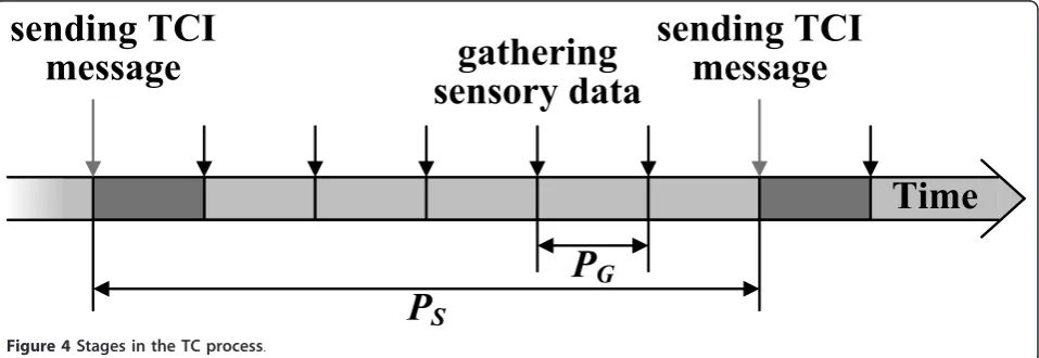
Figure 4 shows the stages in our algorithm. First, the sink nodes0 (in Layer 0) broadcasts a TCI message for the current round, of lengthPS. This message is

com-posed by the sink node, using information gathered from all the nodes in the WSN before the setup period. We assume that PSis even greater than PGbecause our

target is long-term WSN in which layer selection is rarely occurred. Thus the overhead of flooding TCI message is little enough to be negligible.

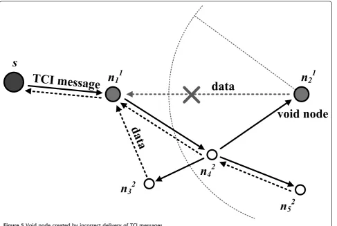
A noden_ican determine its layerjfrom this informa-tion, and can be written nj_i. If a node nj_i receives another TCI message from a node in a layer higher than j, it re-determines its layer from the new TCI message; but this layer must not be higher than the layer of the sender of the TCI message. Otherwise, the node would become void, as shown in Figure 5, and the data sent to it from lower-layer nodes would be lost. After it has determined its layer, a node adds that information to

Layer 0

Layer 1

Layer 2

WSN

n

n

n

n

n

n

n

n

n

n

s

the TCI message it received, and broadcasts the revised message to its neighbors. Repetition of this process makes it possible for all the nodes to determine their own layer. Algorithm 3.2 is a formal statement of this procedure.

Algorithm 1 Layer-based TC algorithm

Require:Sink nodesbroadcasts the TCI message. Require:The layerjof each node is MAX_LAYER Require:s calculates _R¯, the average expected lifetime of all nodes.

Ensure:Determining the layerjfor nj_i

1:if nj_i receives the TCI message from na kthen

2: ifj > athen

3: l¬j

4: j¬a

5: whilej < ldo

6: calculating the estimated lifetime Rj_i of nj_i {Equa-tion (6)}

7: if Rj_i>R¯then

8: broadcasting the TCI message {jis selected as

the new layer for nj_i} 9: return

10: else

11: j¬j+ 1

12: end if 13: end while 14: end if 15:end if

3.3 Layer determination

Each node determines its layer by comparing its expected lifetime with the average lifetime of all the nodes. We will now explain this layer-determination algorithm in detail.

3.3.1 TCI message

All the nodes in the WSN send the information described in Table 1 to the sink nodes, so that it can prepare the TCI message. From this information the sink node calculatesCj, the number of nodes currently in each layer, the average lifetime of all nodes, R, and

alternative route

void node

void node

alternative route

Layer-0 node Layer-1 node Layer-2 node

Figure 3Prevention of void nodes. Our scheme avoids void node problem by using same-layer nodes as a relaying node.

P

G

P

S

gathering

sensory data

Time

sending TCI

message

sending TCI

message

the expected amount of data that each layer should

relay, L¯j_relay. This information is put into the TCI mes-sage; Table 2 describes all the information contained in a TCI message.

3.3.2 How a node selects its layer

A node receiving a TCI message determines its layer by comparing _R¯ with its expected lifetime. This is calcu-lated from the following energy model [21]:

econsume= etrans+ereceive+eelec, (1)

whereetransandereceive respectively are the amount of

energy consumed when the node sends and receives packets, andeelecis the energy consumed by the

electro-nics. If packets are transmitted for P seconds and the

transmission range is tr, the amount of energy

consumed is

P

econsume=Ltransβtrα+

P

(ereceive+eelec), ₍₂₎

where Ltrans is the number of bits in packets

trans-mitted forPseconds,a is the path loss (2≤a≤5), and

b is the energy used by the power amplifier for

trans-mitting 1 bit over a distance of 1 m. Thus we can

calcu-late the energy consumed in one round by a node ni

belonging to layerj, as follows:

eroundji=

P PG

Ljtransβtriα+

PS

(ereceive+eelec). ₍₃₎

TCI message

s

n

1

1

n

2

1

n

4

2

data

n

5

2

n

3

2

data

void node

Figure 5Void node created by incorrect delivery of TCI messages.

Table 1 Node information required in preparing a TCI message

Notation Descriptions

j Number of layers in which_nj

i is present

Rj_i Expected lifetime of _nj

i (in rounds)

Lj_relay Amount of data that nodenj_i should relay on layerjduring one round

Table 2 Information in a TCI message Notation Descriptions

j Number of the layer in which the sender resides

Cj Total number of nodes in each layer

¯

R Expected lifetime of the entire WSN (in rounds)

¯

Lj_relay Amount of data that each layer should relay during one round

Ljtrans is the size of a packet, which is the sum of the

packet header sizeLhead, the amount of data cj_i received

from a lower layer, and the amount of data Lj_relay to be relayed from nodes on the same layer, as follows:

Ljtrans=Lhead+

Ldatacj_i

+Lj_relay, (4)

where cj_i is the number of lower-layer nodes that send data to nj_i. However, we cannot measure the value of cj_i

accurately because it can change with the topology. Therefore we estimate cj_i from hj_i, the number of nodes in each layer that sent data to nj_i during a previous round, andNj, the total number of nodes in each layer, as follows: an average path loss calculated during a previous round

as abecause we can not get an accurate value, then we

use the modified equation to determine the energy con-sumed by node nj_i in layerjduring the current round. The lifetime of nj_i can be calculated from eroundji as

fol-lows:

This computation is repeated for decreasing values of

j: the first value ofj which satisfies Rj_j>R¯ determines

the layer of the node. If this inequality is never satis-fied, the node enters the lowest layerM. Getting nodes to choose their layers dynamically in this way moves nodes with a lot of energy into higher layers, where they will work harder, while nodes that are nearly exhausted go to lower layers, where they can conserve energy.

4 Simulation

We wrote a simulation in C++ to evaluate the perfor-mance of the proposed scheme.

4.1 Simulation environment

From the simulation results, we computed the average lifetime of sensor nodes, and its standard deviation, the average number of data packets transmitted, and the number of dead nodes. We considered a flat network topology, and two, three, and four layers. We simulated

a network of 1,000 nodes at a density of 0.02 to 0.1

nodes/m2, and each test set was run for 6,000 rounds

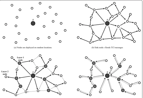
and repeated ten times; then the results use averaged. At the beginning of each round, all nodes were classified into layers (except for the flat topology) using Algorithm 3.2. For example, Figure 6 shows the distribution of nodes in each of three layers. The nodes transmitted data to a sink node using the AODV algorithm [22] at an interval ofP_G. Each sink node broadcasts a TCI mes-sage (similar to a Routing REQuest mesmes-sage in AODV) and all nodes send their data along the reverse of the path that TCI message pass through (similar to a Rout-ing REPly message in AODV). Then the nodes in a higher layer aggregate the data received from the lower-layer nodes with their own data, and transmit all the data to the next node. Figure 7 depicts an example of our simulation process. Each node is powered by a bat-tery of finite life, and dead nodes are immediately replaced with new nodes in the same position. Table 3 contains the important parameters used in our simulation.

4.2 Simulation results

Figures 8 and 9 respectively show the number of packets in the network and the average lifetime of the nodes, measured from our simulation. Figure 9 shows that the layered topologies increased the average lifetime of a node by 2.1 to 22%, compared to the flat topology. In general more layers give a higher performance. Figure 8 shows that the number of packets transmitted decreased by between 30 and 50% as the density of the nodes increased. As node density decreases, the opportunity to receive a TCI message direct from a higher layer decreases. Thus there are fewer nodes in the higher layers, and there is less data aggregation. Conversely, as the density of nodes increases, the fewer packets are transmitted, and the lifetime of the WSN increases, as shown in Figure 8. Our simulation used a simple data

aggregation strategy, in which a node which receives data from a lower layer removes the headers and for-wards the incoming data with its own data. This strategy only eliminates the packet headers received from lower-layer nodes, and thus the average lifetime of the WSN did not increase very greatly. A more efficient aggrega-tion scheme would have much more effect on the amount of data to be sent to upper-layer nodes and we could expect the lifetime of the WSN to improve significantly.

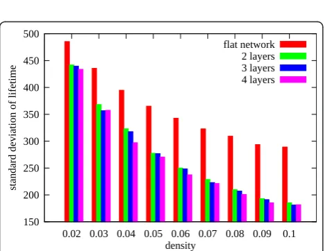
Figure 10 shows the standard deviation of the lifetime of nodes. This is quite high because the nodes closer to the sink node have a shorter lifetimes since they have to relay more data. Depending on the density of the nodes, the standard deviation is reduced by 9 to 36% by our scheme, compared to the flat topology.

Figure 11 shows the cumulative number of dead nodes. Using the flat topology, many nodes died early because of the high standard deviation of lifetime, whereas nodes separated into layers survived longer. This shows how our scheme can prolong the lifetime of a WSN.

Our scheme makes adjusts the number of layers adap-tively, in response to the changing situations of the nodes, up to a specified maximum. Our experiments suggest that performance is usually improved by increas-ing the maximum number of layers, up to a certain number, after which there is no further improvement. For example, in Figure 9, when the density is 0.1, the average lifetime of a node is not increased by going S

(a) Nodes are deployed on random locations. (b) Sink node s floods TCI messages

(c) Nodes select their own layers and reverse paths.

S

(d) Nodes send data to sink node s along the reverse paths

S S

Layer 2 node

Layer 1 node

Figure 7An example of our simulation process.

Table 3 Important simulation parameters

Parameter Value

Number of nodes 1,000

Node density 0.02-0.1

Node placement Random

Amount of data of a packet 100 bytes

Size of header of a packet 40 bytes

Transmission range 10-20 m

Maximum number of layers 1-4

aandbin Equation (2) 3 and 100 pJ/bit/m2

eelecandereceivein Equation (2) 0.003 and 0.066 J

from three layers to four. This suggests that the maxi-mum number of layers should be determined by simula-tion before deployment, since it varies with the number of nodes, their density and distribution.

5 Conclusions

We have proposed a new TC scheme for long-term WSNs. In this scheme, each node deter-mines its own layer, which depends on its residual energy and the cur-rent network status. This allows the WSN to balance itself by allocating energy-intensive roles to energy-rich nodes, thus extending the network lifetime.

As sensors become more efficient, long-term WSNs will become more common, and require more sophisti-cated TC, which we believe can be built on the adaptive layer-based scheme reported in this article.

Acknowledgements

This research was supported partly by Basic Science Research Program through the National Research Foundation of Korea(NRF) funded by the Ministry of Education, Science and Technology(2011-0012996), partly by the Technology Innovation Program funded by the Ministry of Knowledge Economy (MKE) of Korea(10039239), and in part by the ICT at Seoul National University.

Author details

1_{School of Computer Science and Engineering, Seoul National University,}

Seoul, Korea2_{School of Electronic Engineering, Soongsil University, Seoul,} Korea

Competing interests

The authors declare that they have no competing interests.

Received: 30 October 2011 Accepted: 9 May 2012 Published: 9 May 2012

References

1. Y Tseng, SY Ni, YS Chen, JP Sheu, The broadcast storm problem in a mobile ad hoc network. Wireless networks.8(2), 153–167 (2002). doi:10.1023/ A:1013763825347

2. B Chen, K Jamieson, H Balakrishnan, R Morris, Span: an energy-efficient coordination algorithm for topology maintenance in ad hoc wireless Figure 8Number of packets transmitted. The number of gathered

packets in our simulation according to the density of nodes.

Figure 9Average lifetime of nodes. The average lifetime of the nodes measured in our simulation according to the density of nodes.

Figure 10 The effect of node density on the standard deviation of node lifetime. The standard deviation of the lifetime of nodes according to the density of nodes.

networks. Wireless Networks.8(5), 481–494 (2002). doi:10.1023/ A:1016542229220

3. Y Xu, J Heidemann, D Estrin, Geography-informed energy conservation for ad hoc routing. inProceedings of the 7th Annual International Conference on Mobile Computing and Networking:Rome, ACM 2001 70–84 (16-21 July 2001)

4. O Younis, S Fahmy, HEED: a hybrid, energy-efficient, distributed clustering approach for ad hoc sensor networks. Mobile Computing, IEEE Transactions on.3(4), 366–379 (2004). doi:10.1109/TMC.2004.41

5. S Lindsey, C Raghavendra, PEGASIS: Power-efficient gathering in sensor information systems. inProceedings of Aerospace Conference Proceedings

Montana, IEEE 2002.3, 1125–1130 (9-16 March 2002)

6. J Li, P Mohapatra, An analytical model for the energy hole problem in many-to-one sensor networks. inProceedings of IEEE Vehicular Technology Conference:Dallas, IEEE 2005.62, 2721_–2725 (25-28 September 2005) 7. W Heinzelman, A Chandrakasan, H Balakrishnan, Energy-efficient

communication protocol for wireless microsensor networks. inProceedings of the 33rd Annual Hawaii International Conference on System Sciences:

Hawaii, IEEE 2000.2, 10 (4-7 January 2000)

8. E Oyman, C Ersoy, Multiple sink network design problem in large scale wireless sensor networks. inProceedings of IEEE International Conference on Communications:Paris, IEEE.6, 3663_–3667 (24-June 2004)

9. V Shah-Mansouri, A Hamed Mohsenian Rad, V Wong, Multicommodity lifetime routing for wireless sensor networks with multiple sinks. in

Proceedings of IC 2008, IEEE International Conference on Communications:

Beijing, IEEE 2008 3225_–3229 (19-23 May 2008)

10. A Das, D Dutta, Data acquisition in multiple-sink sensor networks. ACM SIGMOBILE Mobile Computing and Communications Review.9(3), 82_–85 (2005). doi:10.1145/1094549.1094561

11. C Buratti, J Orriss, R Verdone, On the design of tree-based topologies for multi-sink wireless sensor networks. inProceedings of the NEWCOM-ACORN Workshop:Vienna 2006 6 (20-22 September 2006)

12. C Buratti, R Verdone, Tree-based topology design for multi-sink wireless sensor networks. inProceedings of PIMRC 2007, IEEE International Symposium on Personal, Indoor and Mobile Radio Communications:Athens, IEEE 2007 1–5 (2-7 September 2007)

13. C Buratti, F Cuomo, S Luna, U Monaco, J Orriss, R Verdone, Optimum tree-based topologies for multi-sink wireless sensor networks using ieee 802.15. 4. inProceedings of VTC 2007, IEEE 65th Vehicular Technology Conference:

Dublin, IEEE 2007 130–134 (22-25 April 2007)

14. J Kim, S Lee, Spanning tree based topology configuration for multiple-sink wire-less sensor networks. inProceedings of ICUFN 2009, the first International Conference on Ubiquitous and Future Networks:Hong Kong, IEEE 2009 122_–125 (7-9 June 2009)

15. Y Fan, Q Chen, J Yu, Topology control algorithm based on bottleneck node for large-scale WSNs. inProceedings of CIS 2009, International Conference on Computational Intelligence and Security:Beijing, IEEE 2009.1, 592–597 (11-14 December 2009)

16. P Ciciriello, L Mottola, G Picco, Efficient routing from multiple sources to multiple sinks in wireless sensor networks. inProceedings of the 4th European conference on Wireless sensor networks:Delft, Springer-Verlag 2007 34–50 (29-31 January 2007)

17. C Intanagonwiwat, D Estrin, R Govindan, J Heidemann, Impact of network density on data aggregation in wireless sensor networks. inProceedings of the 22nd International Conference on Distributed Computing Systems:Vienna, IEEE 2002 457–458 (2-5 July 2002)

18. S Sharma, M Rani, Three-layer architecture model (TLAM) for energy conservation in wireless sensor networks. inProceedings of ICUMT 2009, International Conference on Ultra Modern Telecommunications & Workshops:

St Petersburg, IEEE 2009 1–5 (12-14 October 2009)

19. Z Duan, F Guo, M Deng, M Yu, Shortest Path Routing Protocol for Multi-layer Mobile Wireless Sensor Networks. inProceedings of NSWCTC 2009, International Conference on Networks Security, Wireless Communications and Trusted Computing:Wuhan, IEEE 2009.2, 106_–110 (25-26 April 2009) 20. Z Ming, X Bugong, Layer-based self-organizing topology control for sensor

networks. inProceedings of CCC 2008, 27th Chinese Control Conference:

Kunming, IEEE 2008 516–520 (16-18 July 2008)

21. T Melodia, D Pompili, I Akyildiz, Optimal local topology knowledge for energy efficient geographical routing in sensor networks. inProceedings of INFOCOM 2004, Twenty-third Annual Joint Conference of the IEEE Computer

and Communications Societies:Hong Kong, IEEE 2004.3, 1705–1716 (7-11 March 2004)

22. C Perkins, E Royer, Ad-hoc on-demand distance vector routing. in

Proceedings of WM-CSA 1999, IEEE Workshop on Mobile Computing Systems and Applications:New Orleans, IEEE 1999 90–100 (25-26 February 1999)

doi:10.1186/1687-1499-2012-164

Cite this article as:Yoonet al.:Multi-layer topology control for long-term wireless sensor networks.EURASIP Journal on Wireless

Communications and Networking20122012:164.

Submit your manuscript to a

journal and benefi t from:

7Convenient online submission 7 Rigorous peer review

7Immediate publication on acceptance 7 Open access: articles freely available online 7High visibility within the fi eld

7 Retaining the copyright to your article