R E S E A R C H
Open Access
A study on time-delay rumor propagation
model with saturated control function
Chunru Li
**Correspondence:
[email protected] Huaian Vocational College of Information Technology, Huaian, 223003, People’s Republic of China
Abstract
In this paper, a time-delay rumor propagation model with a saturated control function is established. Regarding time delay as a bifurcation parameter, Hopf bifurcation is studied. By means of the normal form and the center manifold theorem, a formula is put forward to determine both Hopf bifurcation direction and bifurcating periodic solution stability, together with some numerical simulations to illustrate the relevant theoretical results. Simulation results indicate that an appropriate
government control could make periodic oscillation behaviors of the system become steady so as to improve the balance of a social system.
MSC: 34C23; 34D23
Keywords: rumor; spread; delay; Hopf bifurcation
1 Introduction
After an emergency takes place, the government sector serves as the subject of emergency treatment. As far as the government is concerned, the associated contingency plan should be initiated promptly, including emergency supplies distribution, rescue and information release, etc. During emergency processing, a variety of rumors may be spread along with it to affect government image, course of emergency processing and official contingency strategies. The ultimate aim for studies on rumor propagation law and influencing fac-tors is to effectively control and prevent rumors, guide public opinions, and bring down damages caused by rumor propagation. Research on rumor propagation control strategy is exhibited qualitatively in most cases. The exploration into controls over rumor propaga-tion by qualificapropaga-tion has become a hot spot in recent years [–]. As for the corresponding theoretical accomplishments, most of them concentrate on rumor propagation regulation by the government that takes advantage of media, etc. to carry out external environment intervention strategy and individual immunity method.
Through media, etc., the government makes use of external environment intervention strategy to control rumor propagation, and such a method has attracted increasingly more attention from scholars and managers. Study on rumor propagation control is required to sufficiently seize rumor propagation laws, psychological features of receivers, and inter-ventions from the external environment, etc., so as to effectively deal with relevant prob-lems. In recent years, scholars have achieved certain research accomplishments from dif-ferent perspectives and focuses. Reinforcement of media coverage and timely information
release by the government is an effective widely recognized measure for rumor propaga-tion control at present. According to Huo et al. [], factors such as media coverage and governmental information transparency during propagation and diffusion are taken into account to extend the D-K rumor propagation model; moreover, they also utilize the opti-mal control theory to discuss an optiopti-mal control strategy for rumor propagation. Recently, Zhang and Huang [] have presented an -state ICSAR rumor propagation model with government regulation and control. In their opinion, both high and low propagation rates of rumors are able to lead to repeated propagations.
As rumor propagation is similar to infectious disease transmission, the individual immu-nity method for rumor propagation control is derived from the method of immunization against infectious diseases. Many scholars have carried out relevant studies on immuniza-tion strategies of infectious diseases, and rather plentiful research accomplishments have also been obtained [–]. Without any doubt, theoretical guidance and methods for references are provided for effective controls over rumor propagation by means of indi-vidual immunity. In the process of control over infectious diseases, both treatment and immunization play critical roles. In order to prevent and control transmissions of infec-tious diseases such as measles, tuberculosis and flu, treatment is an important and valid approach. As for the classic epidemic model, the cure rate of the infected is deemed to be in direct proportion to the number of such infected people []. Therefore, dynamic prop-erties according to which application of treatment affects these diseases should be studied. The establishment of an appropriate cure function is a problem rather concerned about by scholars at the time of performing theoretical analysis on epidemicity of diseases. In literature [–], they adopt diverse cure functions to probe into controls over epidemic diseases and set up the corresponding epidemic models provided that different medical resources are limited.
Among studies on rumor propagation, regardless of external intervention strategies that are adopted to control it, the control capability of government cannot be enhanced un-limitedly as far as the finiteness of various resources is taken into consideration. Likewise, beneficial from research accomplishments of infectious disease studies, we can use the study on a saturated cure rate of infectious diseases with treatment capacity constraints for references.
Enlightened by research accomplishments above, in this paper, a rumor propagation model that considers government control limits is constructed, and the relevant dynamic properties are also analyzed.
The structure of this paper is arranged as follows. In Section , the model is constructed. In Section , I study the local stability and the existence of Hopf bifurcation through the study of associated characteristic equations. In Section , I study the direction and stability of Hopf bifurcation. In Section , some numerical simulations are given to support our theoretical predictions. Finally, this paper ends with a brief conclusion.
2 The model
This section describes a delayed rumor propagation model. Our goal is trying to create a realistic model which can provide wide insight into predicting and controlling rumor prevalence.
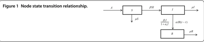
Figure 1 Node state transition relationship.
spreaders (those who are spreading it), and stiflers (those who know the rumor but have ceased communicating it after meeting somebody already informed). For simplicity, we useS(t),I(t) andRto represent the densities of ignorant users, spreading users and stifle users, respectively. To model the propagation of rumor, the following assumptions are imposed:
(i) We consider the recruitment rate of the ignorants is a constant.
(ii) When an ignorant user is infected by spreading users, there is a spreading
incubation period during which the infectious agents develop on networks, and it is only after that time that the infected user becomes himself infectious. Therefore, defining a delay for the spreading incubation period is more appropriate. (iii) Usually, when a rumor is spreading, the government will take effective actions to
control and remove the spreading users.
Our assumption on the dynamical transfer of the nodes is depicted in Figure . As a result, our model can be represented as follows:
⎧ ⎪ ⎪ ⎨ ⎪ ⎪ ⎩
dS
dt =–βSI–μS, dI
dt=βSI–αIR(t–τ) –μI– βI
+αI, dR
dt =αIR(t–τ) + βI
+αI –μR,
()
whereSis ignorant,Iis spreader, andRis stifler.is the recruitment rate of the ignorants, β is the contact rate of ignorant and spreader,μis the death rate of nodes,αis the con-tact rate of spreader and stifler,τ is a non-negative constant representing the spreading incubation period. βI
+αI is a government control function which tends to a saturation level whenIgets large.
In the following, we find all possible non-negative equilibria. Clearly, the system has two feasible non-negative equilibria, namely,
() The boundary equilibriumE(μ, , )representing the state corresponding to the extinction of spreaders and stiflers;
() The interior equilibriumE∗(S∗,I∗,R∗).
At the interior equilibrium point, we must have
⎧ ⎪ ⎪ ⎨ ⎪ ⎪ ⎩
–βSI–μS= , βSI–αIR–μI– βI
+αI = , αIR+ βI
+αI –μR= .
()
Solving the first and the third equation of (), we haveS=
βI+μ andR= βI
(+αI)(μ–αI).
SubstitutingSandRinto the second equation of (), we have
where
A=ααβμ,
A=αβμ+ααμ–αβμ–ααβ,
A=αμ–αμ–βμ–αβ–ββμ+αβμ,
A=βμ–μ–βμ.
()
We make the following assumption:
(H) β–μ–βμ< .
The following results are obvious.
Lemma . If(H)holds,then system()has at least one positive equilibrium E∗(S∗,I∗,R∗),
where S∗=βI∗+μand R∗= βI∗
(+αI∗)(μ–αI∗).
3 Local stability and Hopf bifurcation
In this section, we discuss the local stability and Hopf bifurcation of system () by analyzing the corresponding characteristic equations.
Theorem . IfβS∗–μ+β< holds,then the equilibrium E is locally asymptotically
stable.
Proof It is easily obtained that the characteristic equation corresponding to the equilib-riumEis as follows:
(λ+μ)λ–βS∗+μ–β
= . ()
So, we obtainλ= –μ< andλ=βS∗–μ+β. Therefore, if (H) holds, thenλ< . It
means that the equilibriumEis locally asymptotically stable.
In the following, we consider the stability of the positive equilibriumE∗. At the positive equilibriumE∗, the corresponding characteristic equation is
D(λ) =λ+pλ+pλ+p+
pλ+pλ+p
e–λτ, ()
where
p= μ+βI∗–α,
p= –α
μ+βI∗+μμ+βI∗–α
+IβS∗,
p=βS∗I∗μ–
μ+βI∗μα,
p= –αI∗,
p=αI∗R∗+ααI∗–
μ+βI∗αI∗+αI∗α,
p=
μ+βI∗αI∗R∗+ααI∗+I∗αα
–βS∗I∗α,
α=
β
( +αI∗)
, α=
βαI∗
( +αI∗)
.
Whenτ= , Eq. () becomes
λ+ (p+p)λ+ (p+p)λ+p+p= . ()
By the Routh-Hurwitz criteria, we have the following results.
Lemma . If p+p> ,p+p> , (p+p)(p+p) –p+p> hold,then the positive
equilibrium of system()is locally asymptotically stable withτ = .
Now the effect of the delay on the stability of the positive equilibrium of system () will be discussed. Providing that there is a root of Eq. (), it should satisfy the following equation:
⎧ ⎨ ⎩
–ω+pω= (–pω+p)sinωτ–pωcosωτ,
ω(p+p+p) = –pωsinωτ– (–pω+p)cosωτ.
()
From Eq. (), adding the squared terms for both equations yields
ω+p– p–p
ω+p– pp+ pp–p
ω+p–p= . ()
Letz=ω, then Eq. () becomes
z+p– p–p
z+p– pp+ pp–p
z+p–p= . ()
Denote
h(z) =z+p– p–p
z+p– pp+ pp–p
z+p–p= . ()
Lemma . If the following conditions
αI∗R∗+βS∗μ–αβS∗I∗> , βS∗μ+αβS∗I∗–μα–αI∗R∗–βαα< ()
hold,then Eq. ()has at least a positive root.
Proof From (), we have
p+p=βS∗I∗μ–
μ+βI∗μα+
μ+βI∗αI∗R∗
+μ+βI∗ααI∗–βS∗I∗α,
p–p=βS∗I∗μ–
μ+βI∗μα–
μ+βI∗αI∗R∗
–μ+βI∗ααI∗+βS∗I∗α.
()
If conditions () hold, thenp+p> andp–p< . Obviously,limz→∞h(z) = +∞.
Hence, there is at leastz∈(,∞), so thath(z) = . That is to say, Eq. () has at least a
According to Lemma ., Eq. () has a unique positive root, denoted byz, and thus
Eq. () has a unique positive rootω=√z. By (), we have
cos(ωτ) =
(–pω+p)(p+p+p)ω+pω(–ω+pω)
(pω–p)+ωp
. ()
Thus, if we denote
τj= ω
arccos(–pω
+p
)(p+p+p)ω+pω(–ω+pω)
(pω–p)+ωp
+ jπ ,
j= , , , . . . , ()
then±iωis a pair of purely imaginary roots of () withτ =τj. Clearly, the sequence
{τj}∞
j=is increasing and
lim j→+∞τ
j= +∞. ()
Thus, we can define
τ=τ=min
τj. ()
Lemma . Letλ(τ) =α(τ)±iω(τ)be the root of()nearτ =τj satisfyingα(τj) = , ω(τj) =ω.Suppose that,where is defined by(),the following transversality condition
holds:
d(Reλ(τ)) dτ
τ=τj
= , ()
and the sign of d(Redτλ(τ))|τ=τj
is consistent with that of h (z
).
Proof Denote
R(λ) =λ+pλ+pλ+p, ()
Q(λ) =pλ+pλ+p. ()
Then Eq. () can be written as
R(λ) +Q(λ)e–λτ= , ()
and () can be transformed into the following form:
R(iω)R(i¯ ω) +Q(iω)Q(i¯ ω) = . ()
Thus, together with () and (), we have
Differentiating both sides of Eq. () with respect toω, we obtain
ωhω=iR(iω)R(i¯ ω) –R(iω)R¯(iω) –Q(iω)Q(i¯ ω) +Q(iω)Q¯(iω). ()
Ifiωis not simple, thenωmust satisfy
d dλ
R(λ) +Q(λ)e–λτ
λ=iω
= , ()
that is,ωmust satisfy
R(iω) +Q(iω)e–iωτ–τ
Q(iω)e–iωτ= . ()
With Eq. (), we have
τ=
Q(iω)
Q(iω)
–R (iω
)
R(iω)
.
Thus, by () and () we obtain
Im(τ) =Im
Q(iω)
Q(iω)
–R (iω
)
R(iω)
=Im
Q(iω)Q(i¯ ω)
Q(iω)Q(i¯ ω)
–R (iω
)R(i¯ ω)
R(iω)R(i¯ ω)
=Im
Q(iω)Q(i¯ ω) –R(iω)R(i¯ ω)
R(iω)¯R(iω)
=–i[Q (iω
)Q(i¯ ω) –R(iω)R(i¯ ω) –Q¯(iω)Q(iω) +R¯(iω)R(iω)]
R(iω)R(i¯ ω)
=ωh (ω
)
|R(iω)|
.
Sinceτis real, i.e.,Im(τ) = , we haveh(ω) = .
We get a contradiction to the condition h(ω)= . This proves the first conclusion. Differentiating both sides of Eq. () with respect toτ, we obtain
R(λ) +Q(λ)e–λτ–τQ(λ)e–λτdλ
dτ –λQ(λ)e
–λτ
= , ()
which implies
dλ dτ =
λQ(λ)
R(λ)eλτ+Q(λ) –τQ(λ)=
λQ(λ)[R¯(λ)eλτ+Q¯(λ) –τQ(¯ λ)] |R(λ)eλτ+Q(λ) –τQ(λ)|
=λ[–R(λ)R¯
(λ)eλτ+Q(λ)Q¯(λ) –τ|Q(λ)|]
|R(λ)eλτ+Q(λ) –τQ(λ)| .
It follows together with () that
d(Reλ(τ)) dτ
τ=τ,λ=iω
=Re{λ[–R(λ)R¯
=iωn[–R(iωn)R¯
(iωn) +Q(iωn)Q¯(iωn) +R(iωn)R(i¯ ωn) –Q(iωn)Q(i¯ ωn)] |R(λ)eλτ+Q(λ) –τQ(λ)|
= ω
h(ω)
|R(λ)eλτ+Q(λ) – τQ(λ)| =
ωh(z)
|R(λ)eλτ+Q(λ) – τQ(λ)|= .
Clearly, the sign of d(Redτλ(τ))|τ=τis determined by that ofh(z).
From the above analysis, we have the following theorem.
Theorem . From Lemmas.-.,the following statements are true:
(i) Whenτ∈[,τ),the positive equilibrium point of()is asymptotically stable; (ii) The Hopf bifurcation occurs atτ =τ.That is,system()has a branch of periodic
solutions bifurcating from the positive equilibrium nearτ=τ.
4 Direction and stability of Hopf bifurcation
In this section, we derive explicit formulae to determine the properties of the Hopf bi-furcation at critical valueτj by using the normal form theory and the center manifold reduction developed by [].
First, we let
f()=–βSI–μS, f()=βSI–αIR(t–τ) –μI– βI +αI
,
f()=αIR(t–τ) + βI +αI
–μR,
fij()=∂ i+jf()
∂Si∂Ij, f
()
ijlk =
∂i+j+l+kf()
∂Si∂Ij∂Rl∂Rk, f
()
ijl =
∂i+j+lf()
∂Ii∂Rj∂Rl.
()
Denoteτjbyτ∗and introduce the new parameterμ=τ–τ∗. Normalize the delayτby the time-scalingt→t/τ. Denote
U(t) =S(t),I(t),R(t)T,
then system () can be rewritten as an abstract differential equation in the phase space
C=C([–τ, ],Rn) of the form
dU(t) dt =L
τ∗(Ut) +F(Ut,μ), ()
where
Ut(θ) =U(t+θ), –τ≤θ≤,
L(γ)(φ) =μ
⎛ ⎜ ⎝
–(βI∗+μ)φ() –βS∗φ()
βI∗φ() +αφ() –αI∗φ(–τ)
(αR∗+α)φ() –μφ() +αI∗φ(–τ) ⎞ ⎟
⎠, ()
and
q(ϕ,μ) =τ∗+μ
⎛ ⎜ ⎝
i+j=i!j!f ()
ij ϕi()ϕ
j
()
i+j+l+k=i!j!l!k!f ()
ijlkϕi()ϕ
j
()ϕl()ϕk(–)
i+j+l=i!j!l!f ()
ijl ϕi()ϕ
j
()ϕl(–) ⎞ ⎟
⎠+h.o.t., ()
forϕ= (ϕ,ϕ,ϕ)T∈C.
Then the linearized system of () at the positive equilibrium is
dU(t) dt =L
τ∗(Ut). ()
Based on the discussion in Section , we can easily know that forτ=τ∗, the characteristic equation of () has a pair of simple purely imaginary eigenvalues={iωτ∗, –iωτ∗}.
LetC:=C([–, ],R), consider the following FDE onC:
˙
z=Lτ∗(zt). ()
Obviously,L(τ∗) is a continuous linear function mappingC([–, ],R) intoR. By the
Riesz representation theorem, there exists a × matrix functionη(–≤θ≤), whose elements are of bounded variation such that
Lτ∗(ϕ) =
–
dηθ,τ∗ϕ(θ) forϕ∈C. ()
In fact, we can choose
ηθ,τ∗=τ∗
⎛ ⎜ ⎝
–(βI∗+μ) –βS∗
βI∗ α
αR∗+α –μ ⎞ ⎟ ⎠δ(θ)
–τ∗
⎛ ⎜ ⎝
–αI∗ αI∗
⎞ ⎟
⎠δ(θ+ ), ()
whereδis the Dirac delta function.
LetA(τ∗) denote the infinitesimal generator of the semigroup induced by the solutions of (), and letA∗be the formal adjoint ofA(τ∗) under the bilinear pairing
(ψ,φ) =ψ(),φ()–
– θ
ξ=
ψ(ξ–θ)dη(θ)φ(ξ)dξ
=ψ(),φ()+τ∗
–
ψ(θ+ )
⎛ ⎜ ⎝
–αI∗ αI∗
⎞ ⎟
⎠φ(θ)dθ ()
forφ∈C,ψ∈C∗=C([, ],R). ThenA(τ∗) andA∗are a pair of adjoint operators. From
adjoint operators. LetPandP∗be the center spaces, that is, the generalized eigenspaces ofA(τ∗) andA∗ associated with, respectively. ThenP∗ is the adjoint space ofPand
dimP=dimP∗= . Direct computations give the following results.
∗(s) =q(s) –q(s)
i =
⎛ ⎜ ⎝
Im{e–iωτ∗s} Im{σ∗e–iωτ∗s} Im{σ∗e–iωτ∗s}
⎞ ⎟ ⎠
=
⎛ ⎜ ⎝
–sinωτ∗s
ωcosωτ∗s–(βI∗+μ)sinωτ∗s βI∗
–(βS∗I∗–ω–α(βI∗+μ))sinωτ∗s+ω(βI∗+μ–α)cosωτ∗s βI∗(αR∗+α)
⎞ ⎟ ⎠
fors∈[, ]. From (), we can obtain (∗,) and (∗,). Note that
(q,p) =
∗,
–∗,
+i∗,
+∗,
and
(q,p) = +σσ∗+σσ∗–τ∗αI∗
σσ∗–σσ∗
e–iωτ∗:=D∗.
Therefore, we have
∗,
–∗,
=ReD∗,
∗,
+∗,
=ImD∗.
Now, we define (∗,) = (j∗,k) (j,k= , ) and construct a new basisψforQby
= (,)T=
∗,–∗.
Obviously, (,) = I×, the second order identity matrix. In addition, define f=
(ξ,ξ,ξ), where
ξ=
⎛ ⎜ ⎝
⎞ ⎟
⎠, ξ=
⎛ ⎜ ⎝
⎞ ⎟
⎠, ξ=
⎛ ⎜ ⎝
⎞ ⎟ ⎠.
Letc·fbe defined by
c·f=cξ+cξ+cξ
forc= (c,c,c)T,cj∈R(j= , , ).
Then the center space of linear equation () is given byPCNC, where
PCNϕ=,ϕ,f
·f, ϕ∈c, ()
andC=PCNC⊕PSC, herePSCdenotes the complementary subspace ofPCNCand·,·is the Euclidean product.
LetAτ∗be defined by
Aτ∗ϕ(θ) =ϕ˙(θ) +X(θ)
whereX: [–, ]→B(X,X) is given by
X(θ) = ⎧ ⎨ ⎩
, –≤θ< ,
I, θ= . ()
ThenAτ∗is the infinitesimal generator induced by the solution of (), and () can be rewritten as the following operator differential equation:
˙
Ut=Aτ∗Ut+XF(Ut,μ). ()
Using the decompositionC=PCNC⊕PSCand (), the solution of () can be rewritten as
Ut=
x(t)
x(t)
·f+h(x,x,μ), ()
where
x(t)
x(t)
=,Ut,f
, ()
andh(x,x,μ)∈Pscwithh(, , ) =Dh(, , ) = . In particular, the solution of () on
the center manifold is given by
Ut∗=
x(t)
x(t)
·f+h(x,x, ). ()
Settingz=x–ixand noticing thatp=+i, then () can be rewritten as
Ut∗=
z+z¯ i(z–¯z)
·f+w(z,¯z) =
(pz+p¯z)¯ ·f+W(z,¯z), ()
whereW(z,z) =¯ h(z+z¯, –z–iz¯, ). Moreover, by [],zsatisfies
˙
z=iωτ∗z+g(z,z),¯ ()
where
g(z,z) =¯ () –i()
FUt∗, ,f
. ()
Let
W(z,z) =¯ W
z
+Wz¯z+W ¯ z
+· · · ()
and
g(z,z) =¯ g
z
+gz¯z+g ¯ z
SinceW(θ),W(θ) forθ∈[–, ] appear ing, we still need to compute them. It
fol-lows easily from () that
˙
W(z,z) =¯ Wz˙z+W(˙zz+z˙z) +W¯z˙z+· · · ()
and
Aτ∗W=Aτ∗W
z
+Aτ∗Wzz¯+Aτ∗W ¯ z
+· · ·. ()
In addition, by [],W(z(t),¯z(t)) satisfy
˙
W=Aτ∗W+H(z,z),¯ ()
where
H(z,z) =¯ H
z
+Hz¯z+H ¯ z
+· · ·
=XF
Ut∗, –,XF
Ut∗, ,f
·f,
()
withHij∈PSC,i+j= . Thus, from () and ()-(), we can obtain that
⎧ ⎨ ⎩
(iωτ∗–Aτ∗)W=H,
–Aτ∗W=H.
()
Notice thatAτ∗has only two eigenvalues±iωτ∗with zero real parts, therefore, () has
a unique solutionWij(i+j= ) inPSCgiven by
⎧ ⎨ ⎩
W= (iωτ∗–Aτ∗)–H,
W= –A–τ∗H.
()
From (), we know that for –≤θ< ,
H(z,¯z) = –(θ)()FUt∗, ,f
·f
= –
p(θ) +p(θ)
,
p(θ) –p(θ)
i ()()
×FUt∗, ,f
·f
= –
p(θ)
() –i()
+p(θ)
() +i()
×FUt∗, ,f
·f
= –
gp(θ) +g¯p(θ)
z·f–
gp(θ) +g¯p(θ)
z¯z·f+· · ·.
Therefore, for –≤θ< ,
H(θ) = –
gp(θ) +g¯p(θ)
·f, ()
H(θ) = –
gp(θ) +g¯p(θ)
and
Using the definition ofAτ∗and combining () and (), we get
–
From the above expression, we can see easily that
E=
By a similar way, we have
˙
Similar to the above, we can obtain that
×
⎛ ⎜ ⎜ ⎜ ⎜ ⎜ ⎜ ⎜ ⎜ ⎝
f()+f()(σ+σ¯) +f()σσ¯
f() +f() σσ¯+f() σσ¯+f() σσ¯+f() (σ+σ¯)
+f()(σ+σ¯) +f() (σe–iωτ ∗
+σ¯eiωτ ∗
) +f()(σσ¯+σ¯σ)
+f()(σσ¯eiωτ ∗
+σ¯σe–iωτ ∗
) +f() (σσ¯eiωτ ∗
+σ¯σe–iωτ ∗
) f()σσ¯+f()σσ¯+f()σσ¯+f()(σσ¯+σ¯σ)
+f()(σσ¯eiωτ ∗
+σ¯σe–iωτ ∗
) +f()(σσ¯eiωτ ∗
+σσ¯e–iωτ ∗
)
⎞ ⎟ ⎟ ⎟ ⎟ ⎟ ⎟ ⎟ ⎟ ⎠
.
So far,W(θ) andW(θ) have been expressed by the parameters of system ().
There-fore,gcan be expressed explicitly.
Theorem . System()has the following Poincaré normal form: ˙
ξ=iωτ∗ξ+c()ξ|ξ|+o
|ξ|,
where
c() =
i ωτ∗
gg– |g|–|g|
+g ,
so we can compute the following results:
σ= –
Re(c())
Re(λ(τ∗)),
β= Re
c()
,
T= –
Im(c()) +σIm(λ(τ∗))
ωτ∗
,
which determine the properties of bifurcating periodic solutions at the critical valuesτ∗, i.e.,σdetermines the directions of the Hopf bifurcation:ifσ> (σ< ),then the Hopf
bifurcation is supercritical(subcritical)and the bifurcating periodic solutions exist forτ> τ∗;βdetermines the stability of the bifurcating periodic solutions:the bifurcating periodic
solutions on the center manifold are stable(unstable)ifβ< (β> );and Tdetermines
the period of the bifurcating periodic solutions:the periodic increase(decrease)if T>
(T< ).
5 Numerical simulation
In this section, numerical simulations of some examples are presented to illustrate the theoretical results.
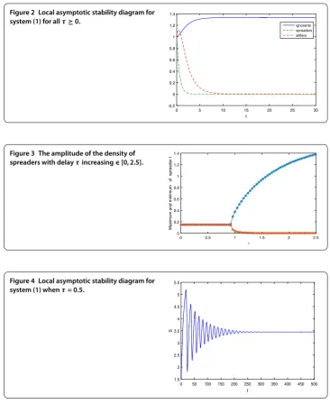
5.1 Stability of the boundary equilibriumE1
Let the parameters of system () be= .,β= .,β= .,α= .,μ= ., andα= ..
Calculation reveals that the boundary equilibrium of system () is (., , ). Obviously, condition (H) holds. According to Theorem ., system () is locally asymptotically stable
Figure 2 Local asymptotic stability diagram for system (1) for allτ≥0.
Figure 3 The amplitude of the density of spreaders with delayτincreasing∈[0, 2.5].
Figure 4 Local asymptotic stability diagram for system (1) whenτ= 0.5.
5.2 Stability and Hopf bifurcation of system (1)
Let = ., β = ., β = ., α = .,μ= ., α= .. Calculation reveals that the
positive equilibrium of system () is (., ., .) and the critical value is τ= .. Figure gives the maximum and minimum of the density of spreaders for
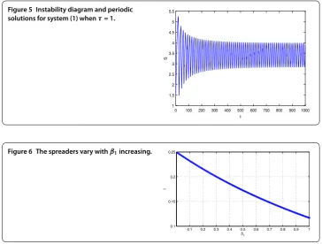
Figure 5 Instability diagram and periodic solutions for system (1) whenτ= 1.
Figure 6 The spreaders vary withβ1increasing.
In addition, whenτ =τ= ., we getc() = –. + .i,σ= –Re–.(λ(τ∗))=
. > ,β= Re(c()) < . According to Theorem . in Section , the bifurcated
periodic solutions of system () whenτ= . in the whole phase space are orbitally
asymptotically stable, and the Hopf bifurcation is supercritical forσ> .
5.3 Effect of the government adjustment power
Taking the same parameters as in Section ., butβ varies in [, ], the corresponding
situations of spreaders are shown in Figure . Numerical evidence shows that with the increase of the adjustment powerβ, the adjustment power makes the population of the
spreaders reduced. This is to say, if the government uses TV (the most popular and believ-able media in China) to announce the truth, the population of the spreaders will reduce immediately.
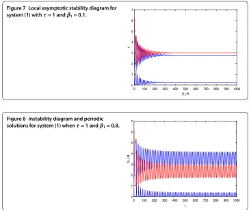
In addition, if we letτ= andβ= ., then the positive equilibrium is locally
asymp-totically stable (see Figure ). However, if we letβ= ., then the positive equilibrium
be-comes unstable as is shown in Figure . It means that the government adjustment power has great effect on system ().
6 Conclusions
In this paper, we considered a delayed rumor model with a saturated control function. Through the theoretical analysis and numerical simulation, we found that government adjustment power can affect system’s stability. These can be found in Section ..
Figure 7 Local asymptotic stability diagram for system (1) withτ= 1 andβ1= 0.1.
Figure 8 Instability diagram and periodic solutions for system (1) whenτ= 1 andβ1= 0.8.
In summary, our study contributes to rumor management by offering an interplay model between rumor spreading and government adjustment. According to the transmission of the rumor, the government should use TV (the most popular and believable media in China) to announce the truth, then the population of the spreaders will be reduced immediately.
Acknowledgements
The work is sponsored by Huai’an agricultural products trading public technical service business construction (BM2012043).
Competing interests
The authors declare that they have no competing interests.
Authors’ contributions
All authors read and approved the final manuscript.
Publisher’s Note
Springer Nature remains neutral with regard to jurisdictional claims in published maps and institutional affiliations.
Received: 22 May 2017 Accepted: 9 August 2017
References
1. Huo, L, Lin, T, Fan, C, Liu, C, Zhao, J: Optimal control of a rumor propagation model with latent period in emergency event. Adv. Differ. Equ.2015(1), 54 (2015)
2. Nekovee, M, Moreno, Y, Bianconi, G, Marsili, M: Theory of rumour spreading in complex social networks. Physica A 374(1), 457-470 (2007)
3. Huang, J, Jin, X: Preventing rumor spreading on small-world networks. J. Syst. Sci. Complex.24(3), 449-456 (2011) 4. Rabajante, JF, Umali, RED: A mathematical model of rumor propagation for disaster management. J. Nat. Stud.10(2),
61-70 (2011)
6. Huo, L, Huang, P, Guo, C: Analyzing the dynamics of a rumor transmission model with incubation. Discrete Dyn. Nat. Soc.2012(2012)
7. Moreno, Y, Nekovee, M, Pacheco, AF: Dynamics of rumor spreading in complex networks. Phys. Rev. E, Stat. Nonlinear Soft Matter Phys.69(6 Pt 2), 066130 (2004)
8. Zanette, DH: Dynamics of rumor propagation on small-world networks Phys. Rev. E, Stat. Nonlinear Soft Matter Phys. 65(1), 041908 (2001)
9. Nekovee, M, Moreno, Y, Bianconi, G, Marsili, M: Critical threshold and dynamics of a general rumor model on complex networks. Eur. J. Gastroenterol. Hepatol.27(Supplement s3), 29-33 (2005)
10. Zhang, W, Tang, Y, Wu, X, Fang, JA: Synchronization of nonlinear dynamical networks with heterogeneous impulses. IEEE Trans. Circuits Syst. I, Regul. Pap.61(4), 1220-1228 (2014)
11. Huo, L, Huang, P: Study of the impact of science popularization and media coverage on the transmission of unconfirmed information. Syst. Eng. Theory Pract.34(2), 365-375 (2014)
12. Zhang, N, Huang, H, Su, B, Zhao, J, Zhang, B: Dynamic 8-state ICSAR rumor propagation model considering official rumor refutation. Physica A415, 333-346 (2014)
13. Cohen, R, Havlin, S, Ben-Avraham, D: Efficient immunization strategies for computer networks and populations. Phys. Rev. Lett.91(24), 247901 (2003)
14. Liu, Z, Lai, Y-C, Ye, N: Propagation and immunization of infection on general networks with both homogeneous and heterogeneous components. Phys. Rev. E, Stat. Nonlinear Soft Matter Phys.67(3), 031911 (2003)
15. Zhu, L, Zhao, H: Dynamical analysis and optimal control for a malware propagation model in an information network. Neurocomputing149, 1370-1386 (2015)
16. Zhu, L, Zhao, H, Wang, X: Bifurcation analysis of a delay reaction–diffusion malware propagation model with feedback control. Commun. Nonlinear Sci. Numer. Simul.22(1), 747-768 (2015)
17. Knapp, RH: A psychology of rumor. Public Opin. Q.8(1), 22-37 (1944)
18. Fisher, DR: Rumoring theory and the Internet: a framework for analyzing the grass roots. Soc. Sci. Comput. Rev.16(2), 158-168 (1998)
19. Pendleton, SC: Rumor research revisited and expanded. Lang. Commun.18(1), 69-86 (1998)
20. Wang, W, Ruan, S: Bifurcation in an epidemic model with constant removal rate of the infectives. J. Math. Anal. Appl. 291(2), 775-793 (2004)
21. Li, XZ, Wang, J, Ghosh, M: Stability and bifurcation of an SIVS epidemic model with treatment and age of vaccination. Appl. Math. Model.34(2), 437-450 (2010)
22. Eckalbar, JC, Eckalbar, WL: Dynamics of an epidemic model with quadratic treatment. Nonlinear Anal., Real World Appl.12(1), 320-332 (2011)
23. Zhang, W, Tang, Y, Miao, Q, Du, W: Exponential synchronization of coupled switched neural networks with mode-dependent impulsive effects. IEEE Trans. Neural Netw. Learn. Syst.24(8), 1316-1326 (2013)
24. Zhou, L, Fan, M: Dynamics of an SIR epidemic model with limited medical resources revisited. Nonlinear Anal., Real World Appl.13(1), 312-324 (2012)
25. Hu, Z, Ma, W, Ruan, S: Analysis of SIR epidemic models with nonlinear incidence rate and treatment. Math. Biosci. 238(1), 12 (2012)