R E S E A R C H
Open Access
Optimization of WLAN associations
considering handover costs
Peter Dely
1*, Andreas Kassler
1, Nico Bayer
2, Hans Einsiedler
2and Christoph Peylo
2Abstract
In wireless local area network (WLAN) hotspots the coverage areas of access points (APs) often overlap considerably. Current state of the art optimization models find the optimal AP for each user station by balancing the load across the network. Recent studies have shown that in typical commercial WLAN hotspots the median connection duration is short. In such dynamic network settings the mentioned optimization models might cause many handovers between APs to accommodate for user arrivals or mobility. We introduce a new mixed integer linear optimization problem that allows to optimize handovers but takes into account the costs of handovers such as signaling and communication interruption. Using our model and extensive numeric simulations we show that disregarding the handover costs leads to low performance. Based on this insight we design a new optimization scheme that uses estimates of future station arrivals and mobility patterns. We show that our scheme outperforms current optimization mechanisms and is robust against estimation errors.
Introduction
Many commercial wireless local area networks (WLANs) are deployed with a considerable overlap between the coverage areas of two adjacent access points (APs). Con-sequently, users often can choose which AP to connect to. In current systems, end users select an AP to associate with typically using the received signal strength indica-tor (RSSI). This leads to unequal resource usage and poor performance. Recently, especially in enterprize WLAN deployments, centralized management schemes became more and more interesting as they allow to exercise more control on the STA/AP associations. However, finding the best AP for a user station (STA) is non-trivial, as it depends on many factors such as signal strength, interfer-ence and load of the AP. Furthermore, the best AP for an STA might change over time, for example due to mobility or time-variant interference of other users.
Finding the best STA/AP selection has been studied extensively [1-6]. However, those optimization models do not consider thecost of reconfiguring the network: If an STA needs to handover from one AP to another AP, the user might experience a temporary disruption of ser-vice during the handover. In addition, signaling messages
*Correspondence: peter.dely@kau.se
1Computer Science Department, Karlstad University, Karlstad, Sweden Full list of author information is available at the end of the article
required for the handover create overhead. In networks with high dynamicity, reoptimizing the network at every change might lead to high costs through network recon-figuration and to low long term user download rates. Recent measurements have shown that in particular pub-lic WLAN hotspots exhibit a high dynamicity due to short user inter-arrival times and short session durations [7]. User mobility is another cause of changes in the network. In Figure 1, we highlight the problem of too frequent reconfiguration with a simple example. A user moves inside an area that is covered by the three access points AP1, AP2, and AP3. The user would like to download data from the Internet at as high speed as possible. The signal strength and hence the feasible download rate decreases with the distance from the AP. A common optimization strategy (“Scheme A”) is to use the AP which currently provides the highest RSSI/PHY rate (e.g., used by [8]). In this example, AP1 is used until the user reaches the 54 Mbit/s zone of AP2. From then AP2 is used until it reaches the 54 Mbit/s zone of AP3, when the next han-dover is performed. This strategy however might result in overall low performance, if switching from one AP to another AP incurs some cost, e.g., due to service interrup-tion, because the WLAN client needs to authenticate itself to the network, the channel needs to be switched or TCP sessions have a timeout and need to start in the slow-start
AP1
6 Mbit/s 18 Mbit/s
54 Mbit/s
AP2
6 Mbit/s 18 Mbit/s
54 Mbit/s
6 Mbit/s 18 Mbit/s
54 Mbit/s
AP3
Handover Points Scheme A Handover Point Scheme B
Figure 1Example of a user walking in a hotspot area with coverage from different APs.
phase again. If the user walks fast, he/she might be out of the 54 Mbit/s zone of AP2 before the handover is com-pleted and the download can be resumed again. In that case, it would be better to not use AP2 at all (“Scheme B”), even if the user is at the cell border of AP1 where the signal strength is low.
This example demonstrates that the optimal handover policy (when to handover to which AP) depends on many factors, such as the service disruption duration, the net-work topology, the distance and throughput between APs and STAs and the connection opportunities. Clearly, one difficulty of finding the optimal handover policy is that the best decision in the present depends on the unknown future state of the network (e.g., which AP is in reach at what time).
Related study
Optimizing STA/AP associations has been investigated in a number of works. For example, [4] attempts to char-acterize the capacity region of multi-channel WLANs under different association policies. The authors con-clude that the PHY rate and the load dependent through-put must be considered to achieve high performance. [3] presents a user-centric framework to select an AP and its operational channel. STAs exchange information with APs, which then periodically compute the optimal channel and associations. The authors remark that too frequent reoptimziation results in frequent reassociation which influences the user experience due to the hard break-down in the reassociation process.[3] however does not aim to derive how often to reoptimize. For their simu-lations they reoptimize every 600 s, which seems to be very long in dynamic networks. [9] proposes a constant-factor approximation scheme for max-min fair bandwidth allocation in WLANs. For the online optimization of net-works with STAs joining and leaving the authors adopt a Hysteresis approach. [2] applies an approach, in which a reoptimization is only performed when a time or a load threshold is exceeded. [1] proposes an NP-hard,
non-linear optimization problem and heuristic solution algorithm for computing proportional fair AP association in multi-rate WLANs. [10] presents a MILP formula-tion of the STA/AP associaformula-tion problem and implements an optimization system adapting cell-breathing concepts known from cellular networks. [11-15] propose systems for controlling STA/AP associations using simple heuris-tics. [16] proposes a multi-objective optimization problem that tries to avoid unnecessary handovers. However, all those approaches do not consider the costs for handovers in their optimization models.
Besides deciding when to handover to which AP, opti-mizing the actual handover procedure has been the focus of several works and technical standards. For example, [17] investigates how to optimize the scanning procedure for new APs. IEEE 802.11r [18] reduces the number of MAC layer frames required to perform a handover and thereby allows faster handovers. IEEE 802.21 [19] speci-fies procedures for horizontal and vertical handovers. In this standard, a controller that resides either in the net-work or the client decides when to execute handovers. Handover policies (when to handover to what AP) are not part of IEEE 802.21. IEEE 802.11h [20] describes how WLANs can coexist with radars in 5 GHz band. This standard specifies frames to instruct an STA to switch AP and channels. IEEE 802.11r, IEEE 802.11h, and IEEE 802.21 still require a controller to decide when to do a handover. Nevertheless, as we will outline in the Section ‘Implementation in real networks’ those standards can support the implementation of an optimization scheme and to reduce the cost associated with each handover.
Contributions
1. We develop a new model to derive the optimal association strategy for STAs. The system consists of a collection of APs and STAs. The system state is described by service requests, link capacities and link interference conditions. We start by formulating a Mixed Integer Linear model, which allows to maximize the throughput of users for a given network state (later referred as “Static network model”). Based on this static network model we discuss three simple and commonly found myopic optimization schemes (variants of [14] and [2]). Myopic here means that the schemes do not consider costs of future handovers and only try to optimize the present network state. The first algorithm reoptimizes the network at every state change. The second scheme additionally allows to restrict the number of handovers at each reoptimization step. The third algorithm implements a classical hysteresis scheme, where a reoptimization is only applied if the throughput is improved by a configurable amount. 2. Furthermore we formulate a model (later referred as
“Dynamic model”) that assumes that the future network state is known. By violating the
non-anticipativity constraint (i.e., using future state information), too frequent handovers, or handovers to APs that will soon be used by other STAs can be avoided. In a practical setting, it is of course not possible to know the future network state exactly, as the state depends on random user activity. However, in simulations, where the user activity is determined a-priory, the model provides an upper bound on the solution quality of the three simple schemes that do not require exact information about the future. With extensive numerical simulations we show that with respect to the upper bound the simple schemes perform reasonably well if there is little dynamicity in the network. However, if the network state changes often, e.g., due to user mobility, the schemes all exhibit low performance.
3. Therefore we propose an optimization scheme that uses network state estimates of the immediate future. We show that a simple interpolation from the present network state already greatly improves the performance compared to the above mentioned schemes. Our optimization model thus provides valuable insights for the design of centralized WLAN management systems. The aim of this article is not to show how such estimates of the future can be obtained (for example by using mobility predication), but to show that even if those predictions are inaccurate they can help to improve performance.
The rest of this article is organized as follows: In the Section ‘Static network model’, we model the problem of
finding optimal associations and download rates in a static network setting. In the Section ‘Dynamic network model’, we extend this model to incorporate temporal network state changes, such as re-associations cause by user mobil-ity. In the Section ‘Static optimization’, we discuss in detail the impact of disregarding handover costs in the optimiza-tion model. The Secoptimiza-tion ‘Sliding window-based dynamic optimization’ uses the insights of the Section ‘Static optimization’ to devise a new sliding window based opti-mization model. Finally, we conclude the article with the Section ‘Conclusion’.
Static network model
In this section, we develop an optimization model of the network, which considers the network state at a given point of time, but not the dynamicity of changes. In the Section ‘Dynamic network model ’, we extend this model to a dynamic model to incorporate changes over time.
System model and notation
The network consists of STAs and APs which are con-nected to the Internet. STAs download data from the Internet via the APs. Accordingly, we model the network as a set of STAsS and a set of APsA. Each APa ∈ A is connected to the Internet with a connection of capacity ba. A wireless link between APa ∈ Aand STAs ∈ S is denoted as(a,s). As typical for WLAN devices, we assume that a rate adaption scheme is in place, which chooses the best Modulation and Coding Scheme (MCS) for each link. The corresponding PHY rate of the chosen MCS on link (a,s)is denoted asp(a,s).
Interference between wireless links is modeled using collision domains [21,22]. According to this model two links cannot be active at the same time if they are in the same collision domain. We model the collision domain as a set of colliding links I. The collision domain set I includes the element{(a,s),(a,s)}, if and only if (a,s) is in the collision domain of(a,s)(a,a ∈ Aands,s ∈
S). The model assumes that an external mechanism such as time division scheduling or carrier sensing enforces such policy. The notation used throughout this article is summarized in Table 1.
Variables
Our model aims to compute (1) which STA should use which AP and (2) at what rate an STA can download from the Internet via the chosen AP. Therefore, we introduce a binary variablec ∈ {0, 1} that models the connection between an STA and an AP as follows:
c(a,s)=
1 if STAsis connected to APa
0 otherwise. (1)
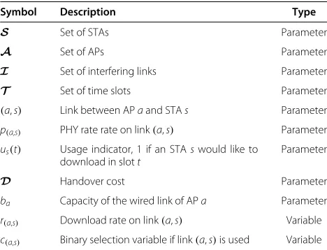
Table 1 Important notation
Symbol Description Type
S Set of STAs Parameter
A Set of APs Parameter
I Set of interfering links Parameter
T Set of time slots Parameter
(a,s) Link between APaand STAs Parameter
ba Capacity of the wired link of APa Parameter
r(a,s) Download rate on link(a,s) Variable
c(a,s) Binary selection variable if link(a,s)is used Variable
r(a,s) ∈ R+. With download rate we refer to the rate that a user can download data with (not considering protocol overheads) and not the PHY rate. In practice, such down-load rates can be enforced by rate shaping at the APs and routers and/or adapting MAC layer parameters [23].
Model constraints
The network is described with the following set of integer-linear constraints:
Equation 2 ensures that an STA is connected to at max-imum one AP. Equation 3 ensures that a station can only download when it is connected. M is a large number (greater than the download rate of any STA). Equation 4 makes sure that all STAs connected to an AP cannot download more than the connection of the AP to the Internet allows. Equation 5 states that the normalized data rate of a link and the links in its collision domain can-not exceedηand thereby guarantees schedulable rates.η models the efficiency of the MAC layer protocol and is smaller or equal than 1 (we useη=1 in the remainder of
the article). Equations 6 and 7 specify the domain of the decision variables.
Solving the model
We aim to maximize thedownload rateof each STA. We hence are confronted with a multi-objective optimization problem, in which the rates of the STAs are the objec-tives. A standard method for solving such problem is to construct a single aggregate objective function (AOF) and maximize this function [24]. The AOF has great impact on fairness and the efficiency of the resource allocation. The often used weighted max-sum AOF might lead to unfair resource allocation and starvation of individual users. In order to enforce fairness, we define the following AOF:
maximizeα+κ
s∈S
a∈A
r(a,s) (8)
where κ is a fairness parameter and α is a continuous variable described through the following additional con-straint:
−
a∈A
r(a,s)+α≤0 ∀s∈S. (9)
Equation 9 states that each STA must receive at least a rate ofα. Whenκis set to 0, the minimum download rate is maximized. However, by the definition of equation 8 it might occur that some download rates are not maxi-mized beyondα, even if they could be increased without decreasingα. By increasingκ, more focus is put on overall network performance and less on fairness. Hence,αmight be lower then. In the rest of the paper we setκ = 10−8 to enforce a high level of fairness and to make sure that download rates are maximized beyondα.
Equations 2–9 constitute a Mixed Integer Linear Pro-gram (MILP) which can be solved with MILP solvers such as CPLEX [25]. We have implemented the model in CPLEX and seen that even for a relatively large network (13 APs and 40 STAs) the problem can be solved within seconds on a normal PC (2.26 GHz Intel Core2 Duo, 4 GB RAM).
Dynamic network model
We proceed by extending the static network model to a dynamic model. The main difference between the static and the dynamic model is that the dynamic model incor-porates a temporal view on the network. For example, the dynamic model considers when an STA joins the network, how the link speed changes over time and when the STA leaves the network again.
Parameters and variables
two slots. The set of slots is denoted withT. Given a slot t∈T,t+1 refers to the slot followingt.
Typically, WLAN hotspot users do not want to down-load data continuously. Users instead downdown-load, e.g., a website and wait a while before issuing a new request. This user activity is modeled with a parameteru:
us(t)=
1 if STAswould like to download in slott 0 otherwise.
(10)
Furthermore, the parameters p and I are now time dependent. We writep(a,s)(t)to describe the PHY on link
(a,s) in slot t. Similarly, I(t) now specifies the set of interfering links in slott.
When a station connects to an AP, it cannot download data immediately. First, control messages for authenti-cation, encryption key negotiation and address assign-ment need to be exchanged. Consequently, we distinguish between two states “connecting” and “connected”. The cor-responding binary variables ˆcand care hence given as:
ˆ
A STAscan only download data when it is in the con-nected state. A STA can only enter the connected state after it has been in theconnectingstate forDa(s)time slots. In other words,Da(s)models the service interruption dura-tion (in time slots) when an STAsperforms a handover to APa.
As an STA cannot be in connected state of one AP and connecting state of an other AP simultaneously, we enforce that the connection state also implies the
con-necting state. Equation 13 is not a linear constraint. We therefore reformulate Equation 13 by replacing the equiv-alence operator with two logical implications and the set expressions with sums:
By using Boolean logic we can reformulate Equation 14 to:
By introducing two binary variablesyandzwe can write Equation 15 as:
Equation 21 ensures that the capacity of the Internet link is not exceeded. Equation 22 ensures that only connected STAs can download. Equation 23 is the capacity constraint of the wireless channel. Equations 24 and 25 state that an STA can only be associated and connected to at maxi-mum one AP in each slot. Furthermore, an STA can only attempt to connect to an AP, if the user is requesting a ser-vice (Equation 26). Finally, Equations 27 and 28 describe the domain of the decision variables.
Objective function
As we are interested in data downloads, the instantaneous download rate of an STA is not so important. The average rate that an STA can achieve during the time it request the service should be maximized instead. Therefore, we specify the following objective function for each STAs:
q(s)= again face a multi-objective optimization problem, which we solve by maximizing a simple aggregate objective func-tion:
maximizeα+κ
s∈S
q(s) (30)
where κ is a fairness parameter and α is a continuous variable described through the following additional con-straint:
−q(s)+α≤0 ∀s∈S. (31)
Equation 16–28 and 31 are now constraints to a stan-dard MILP with Equation 30 as objective function. By solving this MILP we can compute the optimal down-load rates and handover patterns in each time slot, given we know the PHY rates, collision domains and service requests for the whole system run-time.
Depending on the application scenario, other objective functions could be chosen. For example, for multimedia streaming one could try to avoid too long periods with low or zero download rate to minimize video stall times due to buffer underrun. Using a piecewise linear function, time slots with a rate smaller than a threshold can get negative, those larger than a threshold can have positive weight. Evaluating the impact of different objective functions on the solution is however out of the scope of this article.
Static optimization
As the optimization models and goals of [1,3,4,9,10] differ considerable, our goal is here not to compare those approaches directly. We will instead describe three approaches ofwhento invoke the optimization and recon-figure the network. We apply our static model with those approaches and compare the performance to the upper bound provided by the dynamic model (which assumes perfect knowledge of the future).
Invocation strategies Greedy
The Greedy scheme computes the solution to the static
model in every time slot. It does not consider the cur-rent state of an STA (connected or not). It greedily tries to optimize the network configuration in the present state, not considering any implications on the future perfor-mance of the network. If the computed optimal network configuration differs from the current configuration, the required changes to implement the optimal configuration are applied accordingly. This invocation strategy is for example proposed in [14].
In the example network depicted in Figure 1 the greedy scheme produces the same results as “Scheme A”. No interference from other STAs is present and therefore according to the Greedy Scheme it is best to download from the AP with the highest PHY rate.
k-Handover
The k-Handover scheme extends the Greedyscheme by
adding an additional constraint that specifies that at max-imum khandovers can be performed using one slot. As handovers induce service disruption it might be beneficial to limit the number of handovers.
Hysteresis
improvements. In this scheme, the solution quality of the current network configuration αˆ (without changing associations) and the optimal solutionα∗are computed. The optimal solution is then applied if α∗ > α/ˆ f. Typ-ically, f is chosen between 0 and 1. A value close to 0 requires a large improvement over the current solution in order to be applied. This might lead to a small number of handovers, but might operate the network in a subop-timal configuration. In contrast, a value close to 1 might cause a larger number of handovers. This variant of this invocation strategy is for example used in [2].
In the example network of Figure 1, if the user starts walking from the 18 Mbit/s zone of AP1 to the intersec-tion of the 6 Mbit/s zone of AP1 and the 18 Mbit/s zone of AP2, the solutions areα∗= 18 andαˆ =6. Forf <1/3, a handover to AP2 would be triggered.
Evaluation
Next we evaluate the performance of the invocation strategies presented above and the impact of different parameters such as user mobility considering reconfigura-tion cost. Our key findings are that
• User mobility has a significant impact on the
performance of the invocation strategies.
• With low mobility, a Hysteresis based scheme
performs well.
• The impact of the handover cost on performance
depends on the user mobility.
Evaluation settings
We used CPLEX [25] and a set of custom-made simulation scriptsa to numerically evaluate the performance of the different schemes. In each time slot the static optimization problem is solved and the solution is applied according to the invocation strategy under investigation. The size of dynamic model grows proportionally with number of time slots. In order to solve the model fast and to be able to run a large set of different scenarios, thenumber of timeslots should not be too large. A shortslot lengthis a more accu-rate representation of the reality, in which the network state changes continuously and not only at slot bound-aries. However, short slot lengths lead to a large number of slots when simulating a long time period. In our sim-ulations, time slots are1 secondlong and the network is simulated for120 slots. During this time, each user ran-domly generates one traffic request within the first 30 s and aims to download data from the Internet via an AP for at least 50 s. Each simulation was repeated 30×with different random STA positions and mobility patterns.
When an STA arrives at the network, it first connects to the AP with the highest signal strength. Only after connecting, it can receive instructions to handover to a new AP. The performance comparison metric is the
minimum average throughput, i.e.,αin Equation 31. The STA mobility follows the random way-point model with fixed way points: STAs move along the corridors and when they arrive at a junction, they decide randomly which cor-ridor and direction to follow. With this model, synthetic mobility traces were created by randomly placing STAs on the map (Figure 2) of the Computer Science Department of Karlstad University. A total of 13 APs are positioned according to the real deployment and assumed to have Fast Ethernet connections to the Internet (100 Mbit/s). With the Cisco Prime Network Control System software [26] we determined the achievable PHY rates between STAs and APs at each location of the map. In a real net-work, STAs and APs should have an autorate mechanism in place, which allows them to determine the PHY rate. By adjusting the speed of the mobile STAs and the frac-tion of mobile STAs, the dynamicity of the network can be varied.
Evaluation metric and statistical analysis
Our main interest is to compare the different invocation schemes with respect to the upper bound provided by the model in Section ‘Dynamic network model ’. Hence, we use thenormalized minimum throughput α˜ as a perfor-mance metric. Formally,α˜is defined as
˜
α=α/α∗. (32)
Recall thatα denotes the minimum throughput of all stations and the optimal value of α computed with the dynamic network model is calledα∗. Hence, the normal-ized performance ranges between 0 and 1, where a value of 1 means that the respective heuristic is as good as the optimum solution. The plots below show the average (error-bars are standard deviation) of the 30 repetitions.
Impact of user mobility and network size
Handovers of STAs are typically necessary due to user mobility and due to newly arriving STA. To evaluate the impact of both effects, we first simulated a network with 40 STA, of which 0, 10, 20, 30, or 40 STAs are moving at a speed of 1 m/s and the rest are static. The handover cost
Dis 3 for all handovers, i.e., a handover results in 3 time slots where no data can be downloaded.
Figure 2Map of the computer science department and AP locations.
less aggressive when triggering handovers and hence sta-tions are not in the connecting state so often, which is often beneficial for performance.
With no STA mobility, the gap between the heuristics and the optimum is caused by two effects: first, even in absence of mobility, handovers might be required when STAs join or leave the network. The heuristics do not find the best points in time for those handovers. Second, the heuristics maximize the fair throughput in each time slot. In order to maximize the long term average fair through-put, the dynamic model allows temporary unfairness. As
mobility increases the timing of handovers gets more important and hence the performance of the heuristics drops.
The performance of the Greedy and the k-Handover scheme is identical. We found that the k-Handover scheme does not really avoid handovers, it just delays them to the next time slot (if there are alreadykhandovers in the current time slot).
Figure 3Impact of mobility on algorithm performance (D=3, 40 STA).
arrivals/departures and mobility. We now assume that all STAs move with the same speed. Figure 4 shows that an increase in speed results in a decrease of performance. This trend is also due to the higher number of state
changes because of faster mobility and the resulting han-dovers. Generally, if the user mobility gets too high, none of the schemes performs very well. A direct comparison between the schemes shows that the Hysteresis scheme outperforms thek-Handover and the Greedy scheme in 75% of all simulation instances.
Figure 4 furthermore shows that for a fixed speed (e.g., 0 m/s), the performance decreases if the number of STAs in the network is increased. A larger number of STAs causes more dynamicity in the network, e.g., through new STA arrivals. Each time the state of the network changes, the discussed invocation strategies might trigger a han-dover, even if it might be better to remain in the current network configuration for a while and only change the STA/AP associations later.
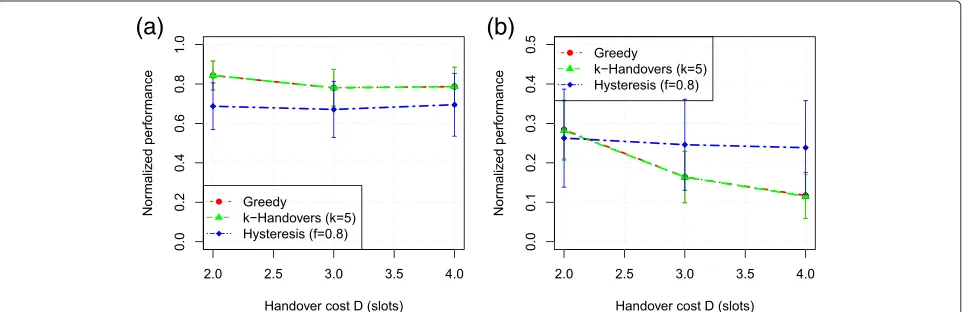
Impact of handover costD
The interruption due to handovers depends on many fac-tors, such as the used hardware and encryption scheme. For commercial enterprize WLANs or hotspots the inter-ruption is in the order of a few hundred milliseconds to a few seconds [27-29]. When further taking into account the interruption due to TCP timeouts and packet losses, 2–4 s are a realistic range [30].
(a)
(b)
(d)
(c)
The impact of the handover cost D depends on the dynamicity of the network. As Figure 5a shows, for han-dover costs between 2–4 slots and static stations, there is almost no impact due to higher handover cost. If sta-tions are not moving, the number of handovers is small and hence the cost of handovers plays no role. However, if stations move (Figure 5a), the handover cost has a consid-erable impact on the performance. In particular with the Greedy and thek-Handovers scheme the normalized per-formance decreases from 28 to 12%. With those schemes, many unnecessary handovers are triggered and stations spend a lot of time performing handovers and connect-ing, instead of downloading data. The Hysteresis performs better in some cases as it avoids a flapping between access points.
We would like to note that a constant normalized per-formance as seen with the Hysteresis scheme does not necessarily reflect a constant absolute throughput. For example, in the case of 1.5 m/s station speed, the normal-ized throughput remains almost constant regardless of the handover cost. The absolute throughput however drops from 2.2 to 1.5 Mbit/s.
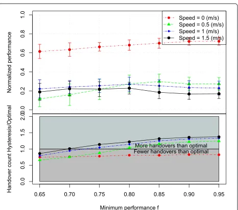
Impact of hysteresis parameter f
Recall, that in the Hysteresis scheme we apply the opti-mal solution, if it is better than the current solution divided by f. Figure 6 shows the impact of f on net-works with different node mobility. The figure confirms the results provided in [31,32]: the optimal Hysteresis margin depends on many factors such as network traffic and channel conditions.
If there is no mobility in the network (speed 0 m/s), only a few handovers are required due to station arrivals. So, even a small improvements due to a handover (which are infrequent in this setting) should be exploited as the net-work state is stable for a longer time afterwards. Hence a largef is better in such a situation. With higher
mobil-ity the opposite is true: smaller values forf are better. For example, when nodes move with 1.5 m/s, f = 0.7 gives best performance and chooses the optimal amount of han-dovers. However, the normalized performance then does not exceed 0.2, showing that not only the number of han-dovers matters. The rate allocation and the actual choice of the STA/AP associations are more important.
Impact of handover limitk
The parameterkdetermines how many handovers can be performed at maximum in each time slot. We evaluate the impact of this parameter for different user mobility patterns. Figure 7 shows that there is almost no influ-ence ofk on the performance. This is not surprising, as thek-Handover scheme only delays handovers to the next time slot (if there are alreadykhandovers in the current time slot). Hence the result of the differentk-s is almost identical.
Discussion
The numerical evaluation has shown that the proposed invocation strategies work well as long as there is no user mobility. In that case, 70–80% of the bound given by the dynamic model are achievable. However, when the users are mobile, the performance quickly drops below 20%. A detailed analysis of the handover patterns has revealed that indeed the reasons for this low performance are too frequent handovers (as illustrated in the motivating exam-ple of the Section ‘Introduction’) or handovers to APs that will soon be used by other STA. Sometimes it is bet-ter, if an STA does not immediately handover to the AP with the highest signal strength, but remains at the cur-rent one (even if the signal strength and the resulting MCS are lower). We apply this insight in the following section, where we develop a sliding window scheme that estimates the immediate future networks states and incorporates this in the handover decisions.
(a)
(b)
Figure 6Impact of hysteresis factorf(30 STA,D=3).
Sliding window-based dynamic optimization In this section, we develop and evaluate a sliding window-based scheme. They key ideas of this scheme are to use predictions of the immediate future and to consider amount of data a STA has already downloaded in the past. This allows to avoid too frequent handovers and to compute a better the rate allocation. The scheme does not include or depend on any specific method to predict the future network state. We show that already a simple prediction method of the future network state is useful, even if the predictions are erroneous. Developing more sophisticated estimation methods are out of the scope of this article.
Figure 7Influence of maximum allowed changes on the performance ofk-Handover (with 30 STA,D=3).
Sliding window method
We denote the current time slot as tc. As shown in Figure 8, we define two windows. The memory window includesWm time slots in the past, the prediction win-dow includes Wp time slots in the future. Furthermore, we define the set of slotsT = {tc,. . .,tc+Wp+1}and
Tm = {tc−Wm−1,. . .,tc−1}.T\tcdenotes the time slots in the prediction window,Tmthe slots in the memory window. We replace Equation 29 with Equation 33 to max-imize the utility duringT, taking into account the already downloaded data duringTm.
q(s)=
t∈Tm
a∈Ar(∗a,s)(t)+
t∈T a∈Ar(a,s)(t)
t∈Tmus(t)+
t∈T us(t)
.
(33)
Withr(∗a,s)(t) (wheret ∈ Tm)we denote the download rate of STAs from AP a during time slots prior to the current time slot. Hence, it is not a variable (since we can-not change the past), but a parameter. The parameters p(a,s)(t)andus(t)for timestc+Wp+1> t> tcare not known and need to be estimated. Different techniques are available to estimate those parameters. Each one comes at different cost and achieves different accuracy. For exam-ple, one could utilize mobility prediction techniques [33] or machine learning techniques such as Support Vector Machines [34] for the parameter estimation. We would like to point out that our approach is independent of the prediction technique.
Evaluation
We evaluated the sliding window method using the setup of the Section ‘Evaluation’ in a network with 10 STA moving at 1.5 m/s. Under those settings the invocation strategies of the Section ‘Evaluation’ reach at maximum 35% of the upper bound. We compare the performance of the sliding window method with different prediction window sizesWp (Wm is set to 120 for all simulations) and prediction errors. We assume that parameters can be estimated with higher accuracy in the immediate future than in distant future. Hence, the probability that a pre-dicted parameter at slott ≥ tcis not equal to the actual parameter can be described as 1−(1−e)t−tc, wheree ∈
Current Time Slot tc
Prediction Window Length=Wp
Time Line Memory
Window Length = Wm
Figure 9Performance of sliding window-based optimization.
[ 0. . .1] models the accuracy of the prediction. Further-more, we implement a simple prediction method, where we set p(a,s)(t) = p(a,s)(tc) and us(t) = us(tc), i.e., we assume that using the present network state will remain unchanged during whole prediction window. We call this estimation “Simple Estimation”.
Figure 9 depicts the performance for different window sizes and error rates. Note thatWp = 120 ande = 0 is equal to the dynamic model, as a window of 120 covers the whole simulation duration. ForWp = 0, all approaches perform equally good, as no prediction is done. As shown in the previous section, the simple Hysteresis achieves 0.35 under same conditions. The increase from 0.35 to 0.5 is due to the memory window, which takes into account how much data has already been downloaded and hence the available resources are distributed among STAs bet-ter. For example, if an STA has already downloaded at a high average rate in the past, its download rate can be decreased in the present and thereby allow other STAs to
download faster. When increasing the prediction window, the performance increases most of the time. Consider the case of e = 0. There is a significant increase between Wp = 0 andWp = 2, 3 or 4. A larger prediction window allows the optimizer to remain connected to an AP with weak signal strength and not handover immediately. Fur-thermore, it avoids to handover to an AP which is used by an other STA in the next slots.
Figure 10 shows those effects with the example of one STA and prediction window sizes of 0, 10, and 20. The figure shows where the STA is connected in which time slot and how many STAs in total are connected to the same AP. With a prediction window of 0, the STA tries to connect to an AP several times, but needs to change again before it can download (because another AP is bet-ter meanwhile). For example, in slot 8 and 9 the STA downloads from AP 9. Then after 9 slots the STA tries to connect to other APs, and only at slot 16 it is connected to AP 7. With larger prediction windows, e.g.,Wp = 10, the STA does not attempt other connections and hence is already connected to AP 7 in slot 13. The example also shows that the load is balanced better with larger predic-tion windows. In this example, with predicpredic-tion window sizes 10 and 20, the STA never shares an AP with other STAs. In contrast, with a prediction window size of 0, the STA needs to share during 4 time slots. The example fur-thermore shows that withWp= 20, fewer handovers are required than withWp =0 orWp =10 and that the STA is in the connected state longer.
Surprisingly, a larger window is not always better. For example on averageWp = 10 is better thanWp = 20. A larger window sometimes results in handovers to accom-modate for a change in the network state in future (e.g., after 17 slots), which is not non-optimal compared to a very large window. However, the smaller window cannot
“see” that network state change, as it is outside the predic-tion window.
Introducing errors to the prediction makes the perfor-mance worse. However, even with a large error probability in the prediction (e = 0.20 means that at 5 slots in the future the state is wrongly estimated with 67% likeli-hood) good performance gains can be achieved. However, it seems not to be beneficial to extend the prediction win-dow to more than 5 slots, as the error probability gets too high then.
The simple estimation method works relatively well for small prediction windows. WithWp = 5 approximately 65% of the normalized performance can be achieved. This is an increase of 15% compared to Wp = 0 and 30% compared to the Hysteresis scheme.
Implementation in real networks
The aim of this article is not to present any practical implementation of the proposed schemes. However, we would like to emphasize that the sliding window scheme can be implemented in enterprise WLANs and public hotspots. For example, [35], [13] or [14] present man-agement architecture proposals for implementing an AP selection scheme in WLANs or mesh connected WLANs. They include central control servers, which collect mon-itoring information and could in principle execute our optimization scheme. IEEE 802.11k [36], a recent IEEE standard that describes the exchange of monitoring infor-mation between APs and STAs, can be used to obtain information about available connection opportunities and interference from the STA. IEEE 802.21 or IEEE 802.11h could be used to trigger handovers.
Conclusion
In this article, we have investigated the AP/STA associ-ation selection and rate control problem under dynamic network conditions. We have demonstrated that disre-garding the costs of handovers and network reconfigura-tion results in performance degradareconfigura-tions of up to 80%. In particular short session durations and user mobility contribute to this performance degradation. As devices withinstant on feature, such as smartphones and tablet PCs, get more common, short sessions and mobility play a more important role.
We have developed an optimization scheme that takes into account estimates of the future network state. By pre-dicting future states and using this information during the optimization better decisions can be done which trans-late into higher performance, even if the predictions are not accurate. Our scheme is independent of the estima-tion method and can therefore be applied in scenarios that favor different estimation methods. The window based model can be adapted for other static optimization mod-els that currently do not take into account the cost of
handovers (for example [3] or [1]). Thereby those models can deliver improved performance in networks with high dynamicity.
Endnote
aAvailable for download at http://www.cs.kau.se/∼pdely/
downloads/
Competing interest
The authors declare that they have no competing interests.
Author details
1Computer Science Department, Karlstad University, Karlstad, Sweden. 2Telekom Innovation Laboratories, Deutsche Telekom, Berlin, Germany.
Received: 14 February 2012 Accepted: 25 July 2012 Published: 16 August 2012
References
1. W Li, Y Cui, S Wang, X Cheng, inWireless Algorithms, Systems, and Applications,vol. 6221 ofLecture Notes in Computer Science,Approximate optimization for proportional fair AP association in multi-rate WLANs. ed. by G Pandurangan, V Anil Kumar, G Ming, Y Liu, Y Li (Springer, Berlin, 2010), pp. 36–46
2. Y Bejerano, SJ Han, L Li, Fairness and load balancing in wireless LANs using association control. IEEE/ACM Trans. Network.15(3), pp. 560–573 (2007)
3. Y Zhu, Q Ma, C Bisdikian, C Ying, User-centric management of wireless LANs. IEEE Trans. Netw. Service Manag.8(3), pp. 165–175 (2011) 4. T Bonald, A Ibrahim, J Roberts, inProceedings of the 7th International
Symposium on Modeling and Optimization in Mobile, Ad Hoc, and Wireless Networks (WiOPT)The impact of association on the capacity of WLANs. (Seoul, Korea, 2009), pp. 1–10
5. L Luo, D Raychaudhuri, H Liu, M Wu, D Li, inProceedings of IEEE WCNC Improving end-to-end performance of wireless mesh networks through smart association. (Las Vegas, USA, 2008), pp. 2087–2092
6. M Abusubaih, A Wolisz, inProceedings of the 10th ACM Symposium on Modeling, analysis, and simulation of wireless and mobile systems, MSWiM’07 An optimal station association policy for multi-rate ieee 802.11 wireless lans. (ACM, New York, NY, 2007), pp. 117–123
7. A Ghosh, R Jana, V Ramaswami, J Rowland, N Shankaranarayanan, in Proceedings of IEEE INFOCOMModeling and characterization of large-scale Wi-Fi traffic in public hot-spots. (Shanghai, China, 2011), pp. 2921–2929 8. Intel Corporation, Intel(R) PRO/Wireless 2915ABG Network Connection
User Guide (2005), ftp://download.intel.com/support/wireless/wlan/ pro2915abg/sb/
9. Y Bejerano, S Han, L Li, Fairness and load balancing in wireless LANs using association control. IEEE/ACM Trans. Network.15(3), pp. 560–573 (2007) 10. P Bahl, M Hajiaghayi, K Jain, S Mirrokni, L Qiu, A Saberi, Cell breathing in
wireless LANs: algorithms and evaluation. IEEE Trans. Mob. Comput.6(2), pp. 164–178 (2007)
11. A Vasan, R Ramjee, T Woo, inProceedings of IEEE INFOCOM Echos—enhanced capacity 802.11 hotspots. (Miami, USA, 2005), pp. 1562–1572
12. S Vasudevan, K Papagiannaki, C Diot, J Kurose, D Towsley, inProceedings of the 5th ACM SIGCOMM Conference on Internet Measurement (IMC) Facilitating access point selection in IEEE 802.11 wireless networks. (USENIX Association, Berkeley, USA, 2005), pp. 26–26
13. N Ahmed, S Keshav, inProceedings of the 2006 ACM CoNEXTSmarta: a self-managing architecture for thin access points. (Lisboa, Portugal, 2006), pp. 9:1–9:12(12)
14. S Krishnamurthy, M Faloutsos, V Mhatre, inProceedings of the 13th annual ACM international conference on Mobile computing and networking,vol. 18, no. 3 MDG: measurement-driven guidelines for 802.11 WLAN design. (Montreal, Canada, 2007), pp. 722–735
Association, Berkeley, CA, USA, 2008), pp. 73–88, [http://dl.acm.org/ citation.cfm?id=1387589.1387595]
16. A Rebai, M Rebai, H Alnuweiri, S Hanafi, inProceedings of IEEE 17th International Conference on Telecommunications (ICT)An enhanced heuristic technique for AP selection in 802.11 handoff procedure. (Doha, Qatar, 2010), pp. 576–580
17. A Mishra, M Shin, W Arbaush, inINFOCOM 2004. Twenty-third Annual Joint Conference of the IEEE Computer and Communications Societies,vol. 1 Context caching using neighbor graphs for fast handoffs in a wireless network. (2004), p. 4, vol. (xxxv+2866)
18. IEEE Standard for Information technology—Local and metropolitan area networks—Specific requirements—Part 11: Wireless LAN Medium Access Control (MAC) and Physical Layer (PHY) Specifications Amendment 2: Fast Basic Service Set (BSS) Transition, inIEEE Std 802.11r-2008 (Amendment to IEEE Std 802.11-2007 as amended by IEEE Std 802.11k-2008)(2008), pp. 1–126 19. IEEE standard for local and metropolitan area networks—Part 21: media
independent handover, inIEEE Std 802.21-2008(2009), pp. c1–301 20. ISO/IEC Standard for Information Technology—Telecommunications and
Information Exchange Between Systems—Local and Metropolitan Area Networks- Specific Requirements—Part 11: Wireless Medium Access Control (MAC) and Physical Layer (PHY) Specifications Amendment 5: Spectrum and Transmit Power Management Extensions in the 5 GHz Band in Europe, inISO/IEC 8802-11:2005/Amd.5:2006(E) IEEE Std 802.11h-2003 (Amendment to IEEE Std 802.11-1999)(2006), pp. c1–60 21. VSA Kumar, MV Marathe, S Parthasarathy, A Srinivasan, Algorithmic
aspects of capacity in wireless networks. SIGMETRICS Perform. Eval. Rev. 33(1), pp. 133–144 (2005). [http://doi.acm.org/10.1145/1071690.1064228] 22. G Cheung, J Lee, SJ Lee, P Sharma, On the complexity of system
throughput derivation for static 802.11 networks. IEEE Commun. Lett. 14(10), pp. 906–908 (2010)
23. SW Kim, BS Kim, Y Fang, Downlink and uplink resource allocation in IEEE 802.11 wireless LANs. IEEE Trans. Veh. Technol.54, pp. 320–327 (2005) 24. R Marler, J Arora, Survey of multi-objective optimization methods for
engineering. Struct. Multidisciplinary Optimiz.26, pp. 369–395 (2004). doi:10.1007/s00158-003-0368-6
25. IBM ILOG CPLEX, http://www.ibm.com/software/integration/ optimization/
26. Cisco Prime Network Control System Series Appliances, http://www.cisco. com/en/US/products/ps11686/index.html
27. A Mishra, M Shin, W Arbaugh, An empirical analysis of the IEEE 802.11 MAC layer handoff process. SIGCOMM Comput. Commun. Rev.33, pp. 93–102 (2003)
28. I Martinovic, FA Zdarsky, A Bachorek, JB Schmitt, inProceedings of the 13th European Wireless Conference (EW2007)Measurement and analysis of handover latencies in IEEE 802.11i secured networks. (Paris, France, 2007) 29. S Kim, S Choi, S kyu Park, J Lee, S Kim, inProceedings of First International
Conference on Communication System Software and Middleware (Comsware)An empirical measurements-based analysis of public WLAN handoff operations. (Delhi, India, 2006), pp. 1–6
30. F Xin, A Jamalipour, TCP throughput and fairness performance in presence of delay spikes in wireless networks. Int. J. Commun. Syst.18(4), pp. 395–407 (2005)
31. CC Lo, MH Lin, inProceedings of International Zurich Seminar on Broadband CommunicationQoS provisioning in handoff algorithms for wireless, LAN. (Zurich, Switzerland, 1998), pp. 9–16
32. M Halgamuge, K Ramamohanarao, H Vu, M Zukerman, inProceedings of IEEE Wireless Communications and Networking Conference (WCNC) 2006, vol. 1 Evaluation of handoff algorithms using a call quality measure with signal based penalties. (Las Vegas, USA, 2006), pp. 30–35
33. L Song, D Kotz, R Jain, X He, Evaluating next-cell predictors with extensive Wi-Fi mobility data. IEEE Trans. Mob. Comput.5(12), pp. 1633–1649 (2006) 34. H Feng, Y Shu, S Wang, M Ma, inProceedings of IEEE International
Conference on Communications (ICC) 2006,vol. 2 SVM-based models for predicting WLAN traffic. (Istanbul, Turkey, 2006), pp. 597–602
35. P Dely, A Kassler, N Bayer, inProceedings of IEEE International Workshop on Wireless Mesh and Ad Hoc Networks (WiMAN 2011)OpenFlow for wireless mesh networks, Hawaii, USA, 2011)
36. IEEE Unapproved Draft Std P802.11v/D7.0Draft STANDARD for Information technology-Telecommunications and information exchange between systems-Local and metropolitan area networks-Specific requirements-Part 11: Wireless LAN Medium Access Control (MAC) and Physical Layer (PHY) specifications Amendment 8: Wireless Network Management. (2009)
doi:10.1186/1687-1499-2012-255
Cite this article as: Dely et al.: Optimization of WLAN associations
considering handover costs. EURASIP Journal on Wireless Communications
and Networking20122012:255.
Submit your manuscript to a
journal and benefi t from:
7Convenient online submission 7Rigorous peer review
7Immediate publication on acceptance 7Open access: articles freely available online 7High visibility within the fi eld
7Retaining the copyright to your article