Lossless Image compression and decompression using Huffman coding

(1)

International Research Journal of Engineering and Technology (IRJET) e-ISSN: 2395-0056

Volume: 02 Issue: 01 | Apr-2015 www.irjet.net p-ISSN: 2395-0072

© 2015, IRJET.NET- All Rights Reserved

Page 240

LOSSLESS IMAGE COMPRESSION AND DECOMPRESSION

USING HUFFMAN CODING

Anitha. S, Assistant Professor, GAC for women, Tiruchendur,TamilNadu,India.

Abstract

-

This paper propose a novel Image

compression based on the Huffman encoding and decoding technique. Image files contain some redundant and inappropriate information. Image compression addresses the problem of reducing the amount of data required to represent an image. Huffman encoding and decoding is very easy to implement and it reduce the complexity of memory. Major goal of this paper is to provide practical ways of exploring Huffman coding technique using MATLAB

.

Keywords - Image compression, Huffman encoding, Huffman

decoding, Symbol, Source reduction…

1. INTRODUCTION

A commonly image contain redundant information i.e. because of neighboring pixels which are correlated and Contain redundant information. The main objective of image compression [1][9] is redundancy and irrelevancy reduction. It needs to represent an image by removing redundancies as much as possible, while keeping the resolution and visual quality of compressed image as close to the original image. Decompression is the inverse processes of compression i.e. get back the original image from compressed image. Compression ratio is defined as the ratio of information units an original image and compressed Compression is performed by three kinds of redundancies. (1) coding redundancy

(2) Spatial or temporal or inter pixel redundancy (3) Psycho visual Redundancy

Compression further divided into predictive and transform coding. Transformed coding means, the large amount of information are transferred into very small number of blocks. One of the best examples of transformed coding technique is wavelet transform. Predictive means based on

the training set (neighbors), reduce some redundancies. Context based compression algorithms are used predictive technique [2][3].

2. HISTORY

Morse code, invented in 1838 for use in telegraphy, is an early example of data compression based on using shorter

codeword’s for letters such as "e" and "t" that are more

common in English. Modern work on data compression began in the late 1940s with the development of information theory. In 1949 Claude Shannon and Robert Fano devised a systematic way to assign codeword’s based on probabilities of blocks. An optimal method for doing this was then found

by David Huffman in 1951.In 1980’s a joint committee ,

known as joint photographic experts group (JPEG) developed first international compression standard for continuous tone images. JPEG algorithm included several modes of operations. Steps in JPEG

1. Color image converted from RGB to YCbCr

2. The resolution of chromo components is reduced by a factor of 2 or 3. This reflects that the eye is less sensitive to fine color details than to brightness details

3. Image is converted into 8X8 matrix

4. DCT, Quantization is applied and finally compressed 5. Decoding is reversible process except quantization is irreversible.

3 . CODING REDUNDANCY:

Rk is distinct random variable, for k=1,2,…L with related probability

Pr(rk)=nk/n

where k=1,2,…L, Kth_{gray level in an image is represented by}

‘nk’and ‘n’ is used to specifiy total number of pixels in the

(2)

International Research Journal of Engineering and Technology (IRJET) e-ISSN: 2395-0056

© 2015, IRJET.NET- All Rights Reserved

Page 241

each pixel in the still image then the average number of bits required to represent each pixel [4] is

Lavg= ∑L_l(r_k_)p_r_(r_k₎

K=1

The average length of the code words is calculated by summing the number of bits used to represent the gray level and the probability that the gray level which placed in an image.

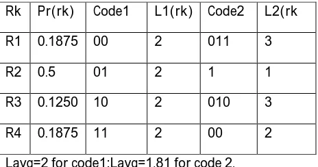
Table 1:Coding redundancy

Rk Pr(rk) Code1 L1(rk) Code2 L2(rk R1 0.1875 00 2 011 3

R2 0.5 01 2 1 1

R3 0.1250 10 2 010 3 R4 0.1875 11 2 00 2 Lavg=2 for code1;Lavg=1.81 for code 2.

Coding redundancy is always present when the gray levels of an image are coded using a binary code. In that table 1, both a fixed and variable length encoding of a four level image is shown. Column two represents the gray level distribution. The 2-bit binary encoding (code1 ) is shown in column 3. It has an average length of 2 bits. The average number of bits required by code2 (in column 5) is

Lavg=∑4_l

2(k)pr(rk)

=3(0.1875)+1(0.5)+3(0.125)+2(0.1875)=1.8125 compression ratio is

Cr =2/1.8125=1.103

4. INTER PIXEL REDUNDANCY:

In order to reduce inter pixel redundancy, the 2-D pixel array normally used for human viewing and interpretation must be transformed into a more efficient format. For example, the difference between adjacent pixels can be used to represent an image. It is called mapping. A simple mapping procedure is lossless predictive coding , eliminates the inter pixel redundancies of closely spaced pixels by extracting and coding only the new information in each pixel. The new information of a pixel is defined as the difference between the actual and predicted value of that pixel.

Fig 1:sample(a) Fig 2: sample(b)

Histogram of Fig 1 & 2

These observations highlight the fact that variable – length coding is not designed to take advantage of the structural relationship s between the aligned matches in Fig2.Although the pixel to pixel correlations are more important in the Fig 1. Because the values of the pixels in either image can be predicted by their neighbors, the information carried by individual pixels is relatively small. visual contribution of a single pixel to an image is redundant; it could be predicted by their neighbors.

5. PSYCHO VISUAL REDUNDANCY:

(3)

© 2015, IRJET.NET- All Rights Reserved

Page 242

Fig 4:original Fig 5 :16 gray level Fig 6 : 16 gray levels/random noise

Consider the image in In fig 4. shows a monochrome image with 256 gray levels. Fig 5 : is the same image after the uniform quantization to four bits or 16 possible levels. Fig 6 is called improved gray-scale quantization. It recognizes the

eye’s inherent sensitivity to edges and breaks them up by

adding to each pixel a pseudorandom number, which is generated from the low-order bits of neighboring pixels, before quantizing the result. In fig 6 removes a great deal of psycho visual redundancy with little impact on perceived image quality.

6. COMPRESSION RATIO:

Compression ratio calculated by the formula Cr=n1/n2

Where n1 is used to represent the total number of bits in an original image and n2 is used to specify the total number of bits in the encoded image. Compression consists of encoding and decoding techniques. Encoding is used to create a unique symbols which are used to specify the original image. The output of encoder is compressed image. The input of decoder is compressed image and the decoder stage is used to get the original image with out getting any error.

Cr=bytes(f1)/bytes(f2);

Where f1 is total number of bytes in the original image and f2 is the total number of bytes in the encoding image.

7 . ROOT MEAN SQUARE ERROR :

To analysis a compressed image, it must be fed into a decoder .f’(x,y) is the decompressed image . It will generated by the decoder.The decoded and the original image is same then the compression is lossless compression otherwise it is lossy. The error energy between the

compressed and the decompressed image is calculated by using the formula

e(x,y)=f’(x,y)-f(x,y)

so the total error between the two images is ∑M-1_∑n-1_[f’(x,y)_-f(x,y)]

x=0 Y=0

and the rms(root mean square)error is used to calculate the error energy between the compressed and the original image and f’(x,y) is the square root of the squared error

averaged over the M*N array , or

rmse=[1/MN∑M-1_∑n-1_[f’(x,y)_{-f(x,y)]2]1/2 ]}

x=0 Y=0

8. HUFFMAN CODES:

Huffman Codes[5] contain small number of possible symbols.All the source symbols are coded one at a time. STEPS :

1.Symbols are placed on the probability values in a decreasing manner.

2. Where there is many number of nodes :

* The new node can be form by merging the two smallest nodes.

* Values ‘1’ or ‘0’ is assigned to each pair of values.

3. From the root we can read the symbols based on their location.

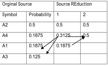
Table 2 : Huffman Source Reduction

Orginal Source Source REduction Symbol Probability 1 2

A2 0.5 0.5 0.5

A4 0.1875 0.3125 0.5 A1 0.1875 0.1875

(4)

International Research Journal of Engineering and Technology (IRJET) e-ISSN: 2395-0056

© 2015, IRJET.NET- All Rights Reserved

Page 243

In table 2, the source symbols are arranged based on their probability values and the values are arranged in decreasing order. To develop the first source reduction , the bottom two probabilities are 0.125 and 0.1875 are joined to create a compound symbol with probability 0.3125. In the first source reduction the compound and its related probability are stored. The probability values are arranged in decreasing order that is from most probable values from the least probable values. This process is repeated until a two symbols which are having the reduced source.

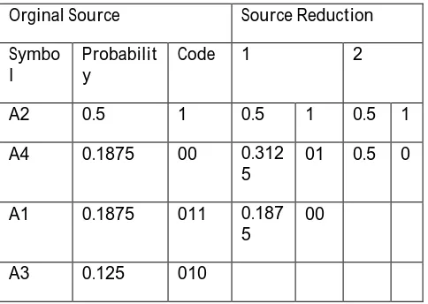
Table 3: Code Assignment Procedures

Orginal Source Source Reduction Symbo

l

Probabilit y

Code 1 2

A2 0.5 1 0.5 1 0.5 1

A4 0.1875 00 0.312 5

01 0.5 0

A1 0.1875 011 0.187 5

00

A3 0.125 010

In the Huffman’s second step consists[ 5] of the reduced source ,which are from the very small source to large one. The reduced source probability symbol 0.5 on the right is generated by merging the two reduced probability symbols in the left. The symbols 0 and 1 is appended to each code for differentiate with each other. This is then repeated for each reduced source until the original source is reached.

Huffman Code tree[6] based on ordered list . The table can be developed based on the tree traversal mechanism. The code for each symbol may be obtain by traveling a direction of the symbol from the root to leaf of the tree. For right

direction the value ‘1’ is assigned and the left direction the

value ‘0’ is assigned. For example a symbol which is reached

by branching left twice, then right once may be represented by the pattern '001'. The figure below depicts codes for nodes of a sample tree.

* / \ (0) (1)

/ \ (10) (11)

/ \ (100) (101)

Once a Huffman tree is built, Canonical Huffman codes, which require less information to rebuild.

9. DEVELOPMENT OF HUFFMAN CODING AND

DECODING ALGORITHM:

At first read the color image. And change the color image into grey level. Then calculate the total number of unique symbols to represent the image. And also calculate the probability values of that symbols. Then create the Symbol table and assign least value to the most probable values. This is called Huffman encoding and Huffman decoding is the reversible process of encoding ,which is used to decompress the image. Finally the quality of the image calculated by root mean square error. If it zero means no difference between the original and decompressed images otherwise some difference is there.

10. ADAPTIVE HUFFMAN CODING

Adaptive huffman coding (Dynamic Huffman coding) is based on Huffman coding, and the symbols are can’t having

no prior knowledge of source distribution. one-pass encoding is used in adaptive huffman [7]. Source symbol have encoded in real time, while it becomes more perceptive to show errors, since just a single loss remains the whole code.

11. IMAGE COMPRESSION TECHNIQUES

The image compression techniques are broadly classified into two categories depending whether or not an exact replica of the original image could be reconstructed using the compressed image .These are:

(5)

© 2015, IRJET.NET- All Rights Reserved

Page 244

11.1 Lossless compression techniques

In lossless compression techniques, the original image can be perfectly recovered form the compressed (encoded) image. These are also called noiseless since they do not add noise to the signal (image).It is also known as entropy coding since it use statistics/decomposition techniques to eliminate/minimize redundancy. Lossless compression is used only for a few applications with stringent requirements such as medical imaging. Following techniques are included in lossless compression:

1. Run length encoding 2. Huffman encoding 3. Dictionary Techniques a)LZ77

b)LZ78 c)LZW

4. Arithmetic coding 5. BitPlane coding

11.2 Lossy compression technique

Lossy schemes provide much higher compression ratios than lossless schemes. Lossy schemes are widely used since the quality of the reconstructed images is adequate for most applications. By this scheme, the decompressed image is not identical to the original image, but reasonably close to it. Following techniques are included in lossy compression: 1.Lossy Predictive coding

a) DPCM b)ADPCM

c)Delta Modulation 2.Transform Coding a)DFT

b)DCT c)Haar d)Hadamard

3.Subband Coding 4.Wavelet Coding 5.Fractal Coding 6.vector Quantization

12. LZ77 :

In the LZ77 approach, the dictionary is simple a portion of the previously encoded sequence. The encoder examines the input sequence through a sliding window. The window consists of two parts, a search buffer that contains a portion of the recently encoded sequence, and a look-ahead buffer that contains the next portion of the sequence to be encoded [8]. The encoder then examines the symbols following the symbol at the pointer location to see if they match consecutive symbols in the look-ahead buffer. The number of consecutive symbols in the search buffer that match consecutive symbols in the look-ahead buffer, starting with the first symbol, is called the length of the match. The encoder searches the search buffer for the longest match. Once the longest match has been found, the encoder encode it with a triple<o,l,c> where o is offset, l is the length of the match, and c is the codeword corresponding to the symbol in the look-ahead buffer that follows the match.

13. LZ78:

LZ77 have the drawback of finite view of the past. LZ78 algorithm to solve this problem by dropping the reliance on the search buffer and keeping an explicit dictionary. This dictionary has to be built at both the encoder and decoder. The input are coded as a double<i,c> with I being an index corresponding to the dictionary entry that was the longest match to the input, and c being the code for the character in the input following the matched portion of the input.

14. LZW :

(6)

International Research Journal of Engineering and Technology (IRJET) e-ISSN: 2395-0056

© 2015, IRJET.NET- All Rights Reserved

Page 245

dictionary as a new entry and assigns it an index value. Compression occurs when the substring, except for the last character, is replaced with the index found in the dictionary. The process then inserts the index and the last character of the substring into the compressed string. Decompression is the inverse of the compression process. The process extracts the substrings from the compressed string and tries to replace the indexes with the corresponding entry in the dictionary, which is empty at first and built up gradually. The idea is that when an index is received, there is already an entry in the dictionary corresponding to that index.

15. ARITHMETIC ENCODING:

Arithmetic coding yields better compression because it encodes a message as a whole new symbol instead of separable symbols .Most of the computations in arithmetic coding use floating-point arithmetic. However, most hardware can only support finite precision [10]. While a new symbol is coded, the precision required to present the range grows. Context-Based Adaptive Binary Arithmetic Coding (CABAC) as a normative part of the new ITU-T/ISO/IEC standard. By combining an adaptive binary arithmetic coding technique with context modeling, a high degree of adaptation and redundancy reduction is achieved. The CABAC framework also includes a low-complexity method for binary arithmetic coding and probability estimation that is well suited for efficient hardware and software implementations.

16. FILE FORMATS WITH LOSSLESS COMPRESSION

• TIFF, Tagged Image File Format, flexible format often

supporting up to 16 bits/pixel in 4 channels. Can use several different compression methods, e.g., Huffman, LZW[11].

• GIF, Graphics Interchange Format. Supports 8 bits/pixel in

one channel, that is only 256 colors. Uses LZW compression. Supports animations.

• PNG, Portable Network Graphics, supports up to 16

bits/pixel in 4 channels (RGB + transparency). Uses Deflate compression (~LZW and Huffman). Good when interpixel redundancy is present.

17. EXPERIMENTAL RESULTS

Consider a simple 4x4 image whose histogram models the symbol probabilities in Table 1. The following command line sequence generates an image by using MATLAB[12][13]. f2=uint8([1 4 6 8;1 6 3 4;2 5 1 4;1 2 3 4])

f2 =

1 4 6 8 1 6 3 4 2 5 1 4 1 2 3 4

>> whos('f2')

Name Size Bytes Class Attributes f2 4x4 16 uint8

Each pixel in f2 is an 8 bit byte; 16 bytes are used to represent the entire image. Function Huffman used to reduce the amount of memory required to represent the image [14][15].

>>c=huffman(hist(double(f2(:)),4)) c =

'01' '1' '001' '000'

To compress f2, code c must be applied at the bit level,with several encoded pixels packed into a single byte .Function mat2huff returns a structure, c1 requiring 528 bytes of memory .

c1=mat2huff(f2) c1=

size: [4 4] min: 32769

hist: [4 2 2 4 1 2 0 1] code: [3639 16066 27296] >> whos('c1')

(7)

International Research Journal of Engineering and Technology (IRJET) e-ISSN: 2395-0056

Page 246

The 16 8-bit pixels of f2 are compressed into two 16-bit words-the elements in field code of c1 is :

hcode=c1.code;

>> dec2bin(double(hcode)) ans =000111000110111 011111011000010 110101010100000

The dec2bin has been employed to display the individual bits of c2.code.

>> f=imread('E:\ph.d\lena512.bmp'); >> c=mat2huff(f);

>> cr1=imratio(f,c) cr1 =1.0692 >> ntrop(f) ans = 7.4455

>> save squeezeimage c; >> load squeezeimage; >> g=huff2mat(c); rmse=compare(f,g) rmse = 0

Overall encoding and decoding process is information preserving; the root mean square error between the original and decompressed images is 0.

Fig 7:Before Huffman Fig 8:After Huffman

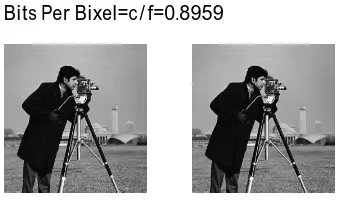
>> f=imread('E:\ph.d\cman.tif'); >> c=mat2huff(f);

>>c1=huff2mat(c); Bits Per Bixel=c/f=0.8959

Fig 9 : Before Huffman Fig 10: After Huffman

18. RESULT ANALYSIS

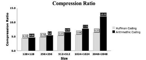
The experimental results of the implemented algorithms, Huffman and arithmetic coding for compression ratio and execution time are depicted in Table 4. As this table shows, on one hand, the compression ratio of the arithmetic coding for different image sizes is higher than the Huffman coding. On the other hand, arithmetic coding needs more execution time than Huffman coding. This means that the high compression ratio of the arithmetic algorithm is not free. It needs more resources than Huffman algorithm.

Table 4. Average of compression results on test image set.

(8)

Page 247

Figure 11. Comparison of compression ratio for Huffma n and arithmetic algorithms using different image sizes

.

19. CONCLUSION :

This image compression method is well suited for gray scale bit map images. Huffman coding suffer from the fact that the uncompress or need have some knowledge of the probabilities of the symbols in the compressed files this can need more bits to encode the file This work may be extended the better compression rate than other compression techniques. The performance of the proposed compression technique using hashing and human coding is performed on GIF,TIFF formats. This technique can be applied on luminance and chrominance of color images for getting better compression.

REFERENCES

[1]Rafael C.Gonzalez,Richard E.Woods,Steven L.Eddins

,”Digital image processing using Matlab “,second

edition.McGraw Hill Education private Limited,,pp.378-380,2013.

[2]Ming Yang & Nikolaos Bourbakis, “ An overview of

lossless digital image compression techniques,”Circuits &

system,2005 48th_{Midwest symposium,vol.2 IEEE,pp}

1099-1102,7-10 Aug,2005.

[3]Khalid sayood ,” Introduction to data compression “

,Third edition,Morgan Kaufmann Publishers,pp. 121-125,2006

[4]Jagadish h.pujar,lohit m.kadlaskar ,“A new lossless

method of image compression and decompression using

Huffman coding techniques” ,Journal of theoretical and

Applied information Technology,

[5] Dr.T.Bhaskara Reddy,Miss.Hema suresh yaragunti,

Dr.S.kiran,Mrs.T.Anuradha “ A novel approach of lossless

image compression using hashing and Huffman coding

“,International Journal of Engineering research and

technology ,vol.2 issue 3,march-2013.

[6]Mridul Kumar Mathur,Seema Loonker,Dr.Dheeraj

saxena,“Lossless Huffman coding technique for image

compression and reconstruction using Binary trees.”IJCTA

,Jan-Feb 2012.

[7].Dr.T.Bhaskar Reddy, S.Mahaboob Basha,

Dr.B.Sathyanarayana and “Image Compression Using Binary

Plane Technique” Library Progress, vol1.27, no: 1, June

-2007, pg.no:59-64.

[8]A.said, “Arithmetic coding “ in lossless Compression

Handbook,k.sayood,Ed.san Diego, CA,USA:Academic ,2003. [9]Anil.K.Jain , “ Fundamentals of digital Image Processing”,PHI publication,pp.483,2001.

[10] Mamta Sharma ,” Compression Using Huffman Coding”,

IJCSNS International Journal of Computer Science and Network Security, VOL.10 No.5, May 2010.

[11]The Scientist and Engineer’s Guide to Digital Signal

Processing by Steven W. Smith.

[12] G.C Chang Y.D Lin (2010) “An Efficient Lossless ECG

Compression Method Using Delta Coding and Optimal

Selective Huffman Coding” IFMBE proceedings 2010,

Volume 31, Part 6, 1327-1330, DOI: 10.1007/978-3-642-14515-5_338.

[13]Wei-Yi Wei,” An Introduction to image compression”.

[14] C. E. Shannon, “Coding theorems for a discrete source

with a delity criterion," in IRE Nat. Conv. Rec., vol. 4, pp. 142-163, Mar. 1959.

BIOGRAPHIES

ANITHA.S received her Bachelor’s degree

in Computer Science from Govindammal Aditanar College for women, Tiruchendur in 2006. She did her Master of Computer Applications in Noorul Islam College of Engineering, Nagercoil.Completed her M.Phil in MS university, Tirunelveli.At present she is Working as an Assistant Prof.in Govindammal Aditanar College for Women, Tiruchendur.