R E S E A R C H
Open Access
Interference characterization and mitigation
benefit analysis for LTE-A macro and small cell
deployments
Víctor Fernández-López
1*, Klaus I Pedersen
1,2and Beatriz Soret
2Abstract
This article presents a characterization of different LTE-Advanced network deployments with regard to downlink interference and resource usage. The investigation focuses on heterogeneous networks (HetNets) with dedicated spectrum for each layer and, in particular, on cases where small cells are densely deployed. Thus, the main interference characteristics of the macro layer and the dense small cell layer are studied separately. Moreover, the potential benefit of mitigating the dominant interferer in such scenarios is quantified as an upper bound gain and its time variability is discussed and evaluated. A dynamic FTP traffic model is applied, with varying amounts of traffic in the network. The results present an uneven use of resources in all feasible load regions. The interference under the dynamic traffic model shows a strong variability, and the impact of the dominant interferer is such that 30% of the users could achieve at least a 50% throughput gain if said interferer were mitigated, with some users reaching a 300% improvement during certain time intervals. All the mentioned metrics are remarkably similar in the macro and small cell deployments, which suggests that densification does not necessarily imply stricter interference mitigation requirements. Therefore, the conclusion is that the same techniques could be applied in both scenarios to deal with the dominant interferer.
Keywords: Interference; Mitigation; Dominant interferer; LTE-Advanced; Macro cell; Small cell
1 Introduction
Interference is one of the main factors that compromise the downlink performance in LTE and LTE-Advanced (LTE-A) networks [1]. As such, it has been the focus of numerous studies since the first LTE network deploy-ments comprising only macro cells. Research on interfer-ence management for macro-cell networks has analysed, among others, aspects such as resource partitioning in the frequency and space domains (e.g., frequency reuse, fractional frequency reuse) [2-4] to improve the signal strength at the mobile terminal or to reduce the interfer-ence. These studies were performed under static traffic models, therefore limiting the time variability of the inter-ference. Hence, the solutions proposed in these investi-gations managed to bring notable benefits while using slow adaptation capabilities. More recently, coordinated
*Correspondence: [email protected]
1Department of Electronic Systems, Aalborg University, Fredrik Bajers Vej 7, 9220 Aalborg, Denmark
Full list of author information is available at the end of the article
multi-point transmission (CoMP) studies have tried to approach these issues in a more dynamic manner [5], by studying procedures with extensive coordination and, for the most part, under the assumption of a fast backhaul, or even fronthaul, with negligible latency [6].
Following these macro-only topologies, research turned to heterogeneous networks (HetNets) as a way to meet the increasing capacity demands in LTE-A networks. Het-Nets comprise a mixture of macro cells and low-power nodes known as small cells. These topologies face a chal-lenging interference problem in cases where the macro and the small cells utilize the same carrier due to the dif-ference in transmission power. Therefore, this inter-layer interference has been the focus of many studies [7-9]. The current trend is pointing to dedicated deployments with higher frequency bands [10] and thus shifting the focus towards intra-layer interference between the same class of nodes. Most of the research on intra-layer interference between small cells in the literature has considered femto cells (home base stations), which present a high risk for
inter-cell interference as the nodes are commonly installed by the users, making up an unplanned network [11,12].
However, current research is contemplating increas-ingly denser small cell deployments in HetNets [13], where intra-layer interference becomes a considerable concern, even in a planned deployment. It has been claimed that denser scenarios exhibit unique interfer-ence characteristics and therefore will require custom-designed solutions for interference mitigation [14]. This study sets out to evaluate this hypothesis and to under-stand how the efforts to manage interference should be steered depending on the topology. In particular, the impact of the strongest interferer and the potential benefit from cancelling it are evaluated. This investigation contin-ues the work begun in [15], which evaluated the behaviour of the intra-layer interference in an LTE-A dense small cell network. The analysis is extended here to a network based on a regular macro-cell deployment, and we delve deeper into the reasons for the observed interference patterns. Both the macro-only and the dense small cell scenarios are examined under a dynamic traffic model with differ-ent amounts of offered traffic. The time evolution of the interference is studied, analysing the required dynamism for interference mitigation solutions in these topologies.
The two scenarios are found to be remarkably simi-lar with regard to these considerations, despite their very different degrees of density. This conclusion fits in with previous studies such as [8] and [16], which found that, assuming an interference-limited network with unbiased cell association and equal path loss exponents for all links, adding base stations does not modify the downlink SINR statistics. As such, similar strategies to manage the inter-ference could be used in the two scenarios analysed in this article, potentially achieving very significant performance gains if the main interferer were ideally mitigated.
The structure of the paper is as follows: Section 2 will introduce a description of the considered network scenar-ios and the traffic model, together with some necessary theoretical considerations for the interference analysis; Section 3 will focus on a description of the system-level simulation settings; Sections 4 and 5 will present the anal-ysis and discussion of the collected statistics and their significance. The article closes with a discussion on future research and the concluding remarks.
2 Setting the scene
2.1 Network model
The majority of the network models found in the litera-ture are either variations of the Wyner model, making up an idealized, regular structure, or are based on stochas-tic geometry, such as Poisson point processes (PPPs) [17]. The 2D Wyner model forms a regular lattice of determin-istic base station positions, in a hexagonal deployment, whereas in the case of the PPP scenarios, the network
positions are random and the structure, irregular. Both methods have a series of advantages and disadvantages. The Wyner model is more tractable but highly ideal and therefore requires extensive simulations to produce real-istic results. On the other hand, the PPP models account better for randomness in the network and allow us to define the notion of a typical user [18]. PPP has also been found to adequately model the user’s positions, both in a macro cell when applied uniformly over the area and in hotspots when used in clustered form. The main disad-vantage of stochastic models is the difficulty in modelling the correlated dependences in node positions, i.e., the fact that the location of a base station is generally dependent on the position of its neighbours [17].
A third option for network modelling comes in the form of realistic (site-specific) scenarios, generally using data from real operator deployments [19]. The main challenge of performing a study in such a scenario is that the repro-ducibility of the results is limited, and that it might not be easy to extract general conclusions that are applicable to other deployments. The Third Generation Partner-ship Project (3GPP) has adopted the use of Wyner and stochastic models in its simulation assumptions [13]. In particular, macro deployments are represented by a regu-lar hexagonal structure, whereas small cells are deployed in clusters according to a PPP with several inter-eNodeB distance constraints.
The two LTE-Advanced network scenarios considered in this study, which are illustrated in Figure 1, follow these characteristics. The network topologies are similar to the ones described in [13]. On the left-hand side of Figure 1, the macro-cell case comprises seven sites with three sectors each. The deployment is regular, with a 500-m inter-site distance. The users are deployed unifor500-mly over the cell area according to a PPP. All the macro cells transmit at the same frequency. The small cell scenario, depicted on the right-hand side of Figure 1, includes three non-overlapping clusters with ten small cells each, mod-elling areas with high traffic density. As shown in the figure, the clusters are delimited by two concentric cir-cles. The cells are randomly placed according to a Poisson point process within the inner circle, with a 50-m radius. There is a minimum distance constraint between small cells of 20 m. The outer circle, with a 70-m radius, rep-resents the area where the users are deployed uniformly according to a PPP (i.e., taking a clustered approach). All the small cells in the network share the same frequency band. It is assumed that the each user connects to the cell corresponding to the strongest received power.
2.2 Traffic model
Figure 1Network topologies. Macro-cell network (left) and dense small cell network (right).
data to transmit. In contrast, finite-buffer models (also known as FTP traffic models) include user arrival (birth) and departure (death) processes, and it is assumed that the users have a limited amount of data to transmit, and they leave the network once they have done so [20]. These models can be of the closed-loop or open-loop types, depending on whether the number of users in the network is fixed or variable, respectively. Both full- and finite-buffer models have been used in 3GPP studies [21]. The finite-buffer model with Poisson arrival has been found to adequately model the arrival of user sessions [22]. It also includes the effect of users not being simultaneously active, thereby introducing fluctuations in the interfer-ence conditions in the network. The full-buffer model is less realistic in its assumption of constantly active users and results in more stable interference patterns. The dif-ference between the models can be significant in dense deployments where the coverage areas are reduced and the cells serve a low number of users. In such a scenario, the full-buffer model would lead to an underestimation of the interference variability, which would seemingly facili-tate the scheduling decision process. In order to properly understand the challenges faced in dense deployments, this study adopts an open-loop dynamic FTP traffic model in which session arrivals are controlled by an average arrival rate,λ, following a homogeneous Poisson process, and each user demands a fixed payload of L bits. The arrival rate λ has different meanings depending on the scenario. In the macro-cell case,λ indicates the average number of users per second per cell area, whereas in the small cell case, it is defined as the average number of users per second per small cell cluster. The offered load Ois defined as the product of the arrival rate and the payload, O=L· λ, and will accordingly adopt different meanings depending on the scenario. Likewise, we define the car-ried load,C, as the average amount of supported traffic in one of the cells (macro scenario) or in one cluster (small
cell scenario). The different interference and performance metrics analysed in this study will be evaluated in relation to the offered and carried loads.
The system is in equilibrium and operates in the feasible load region when the carried traffic matches the offered load, i.e.,C = O. Congestion takes place when the sys-tem cannot support the demanded traffic (C < O) and the session departure rate becomes lower than the rate at which users arrive in the network. The congestion region is unstable and not of interest for the design of a practi-cal interference management solution. Therefore, only the performance in the feasible load region will be considered in this study.
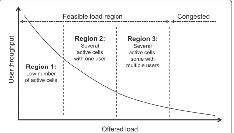
A sketch of the user performance in the feasible region with increasing traffic is presented in Figure 2. This region can be further subdivided in three sub-regions according to the occupation of the cells. Region 1 represents the low load cases, where there are plenty of available resources for the users, which in turn get served quickly and often leave the network before the next arrival. Inter-cell inter-ference can be neglected in this case as the sessions are
very short and the probability of having multiple active cells at the same time is low. In region 2, the offered load has increased, together with the probability of having sev-eral simultaneously active transmitters. However, the load in the cells is still fairly low, with typically one active user per cell. Finally, region 3 represents the case where the load in the network is such that the capacity limit is nearly reached, with a high number of users in some cases and a considerable number of cells transmitting at once.
2.3 Interference mitigation benefit
This section introduces the theoretical analysis that will allow us to evaluate the spectral efficiency gains from mitigating the main interferer. Starting with the most common signal quality measure, the signal-to-interference-plus-noise ratio, SINR (), is defined as
= P n
In+N
, (1)
whereP is the power of the desired signal,nIn
repre-sents the total amount of received interference andN is the background noise. The time variation of the parame-ters in (1) has been kept out of the equation for the sake of notational simplicity.
The dominant interference ratio, DIR (), indicates how significant the role played by the strongest interferer in the total interference profile is. The DIR is defined as
= I1 n
In−I1+N
, I1≥ I2 ≥ . . . ≥ In, (2)
whereI1represents the strongest source of interference.
We can relate the DIR to the potential performance ben-efit that would be obtained assuming ideal cancellation of the main interferer. Under that assumption, the SINR becomes
Taking the ratio of the SINR expressions in (3) and (1), we quantify the improvement from cancelling the strongest interferer as
which is proportional to the DIR value. Finally, the DIR and the SINR can be related to the throughput improve-ment with ideal cancellation of the strongest interferer by applying Shannon’s formula and calculating the ratio of the spectral efficiencies with cancellation, Cc, and
with-out,C,
The packet scheduler determines how resources should be allocated among the multiple users of a cell. Because the packet scheduler performs the resource allocation in an intra-cell fashion, it can only impact the performance in region 3, where there are multiple users within the cell. This study makes use of three different scheduler algo-rithms, all based on the same principle of selecting a user u∗according to a metricMu,
where u is the index of the user, ru is the achievable
throughput for useruin the current Transmission Time Interval (TTI), Ru is the past average throughput and
α,β ∈[ 0, 1] are parameters which control the fairness. The first algorithm, and one of the most commonly used, is Proportional Fair (PF) [23], obtained by
apply-ing α = 1,β = 1 in (6). PF has been found to offer
a good trade-off between scheduling gains and fairness, especially under full-buffer traffic models. In addition, a modified gradient search β-fair scheduler algorithm, known as Generalized PF (GPF), will be included as it was found to be more attractive for scenarios with a birth-death traffic model in [20]. Finally, we will present results for the Blind Equal Throughput (BET) scheduler, with
α = 0,β = 1, targeted to serving users with an equal average throughput [24].
3 Simulation methodology
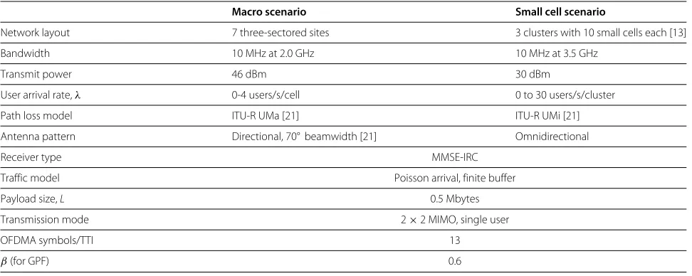
Table 1 Main simulation assumptions
Macro scenario Small cell scenario
Network layout 7 three-sectored sites 3 clusters with 10 small cells each [13]
Bandwidth 10 MHz at 2.0 GHz 10 MHz at 3.5 GHz
Transmit power 46 dBm 30 dBm
User arrival rate,λ 0-4 users/s/cell 0 to 30 users/s/cluster
Path loss model ITU-R UMa [21] ITU-R UMi [21]
Antenna pattern Directional, 70° beamwidth [21] Omnidirectional
Receiver type MMSE-IRC
Traffic model Poisson arrival, finite buffer
Payload size,L 0.5 Mbytes
Transmission mode 2×2 MIMO, single user
OFDMA symbols/TTI 13
β(for GPF) 0.6
In the macro-cell scenario, the cell transmit power is 46 dBm and the antennas have a directional pattern. The carrier frequency is 2 GHz with 10-MHz bandwidth. The arrival rate will range between 0 and 4 users/cluster/s. The stochastic ITU-R urban macro-cell (UMa) radio propagation model is assumed, including different char-acteristics for line-of-sight (LOS) and non-LOS (NLOS) [21]. The LOS case considers shadow fading with a 4-dB standard deviation (σ) and different expressions for the path loss depending on the distance with respect to a breakpoint. The NLOS case has no breakpoint and uses
σ =6 dB for the shadow fading.
In the small cell scenario, all the small cells operate on the same carrier frequency at 3.5 GHz with 10-MHz band-width. The antenna pattern is omnidirectional, and the transmit power is 30 dBm. The arrival rate will be set to values between 0 and 30 users/cluster/s. The path loss model is ITU-R urban micro-cell (UMi) [21], again with different expressions for LOS and NLOS cases. The LOS expression depends on the distance to a breakpoint and appliesσ =3 dB, whereas the NLOS case assumesσ =4 dB.
The remaining simulation parameters are common to
both scenarios. The users demand a L = 0.5 MB
pay-load. Closed loop 2 × 2 single-user MIMO with rank
adaptation is assumed, i.e., corresponding to LTE trans-mission mode-4 [28,29]. Packet scheduling is performed in the time domain only, with one user per TTI [24]. This allows us to increase the number of OFDMA symbols per TTI from 11 to 13 to improve the data rate. The value ofβ in (6) for the GPF scheduler is fixed to 0.6 as rec-ommended in [20]. The link to-system level modelling is according to [25]. The receiver type at the user equipment is MMSE-IRC [30].
4 Performance results
In this section, we will take a look at simulation results which illustrate the interference conditions and achiev-able data rates in the considered scenario, under different traffic loads and scheduling metrics. The first part of the section will focus on establishing the traffic regions as described in Section 2.2 and on a comparison of the scheduling algorithms. Next, we will take a closer look at the load behaviour of the network by examining cell occu-pation statistics. The magnitude and time variability of the interference in the network will be dealt with afterwards, finally offering an estimation of the potential benefits that could be obtained from interference mitigation.
4.1 Traffic load region analysis
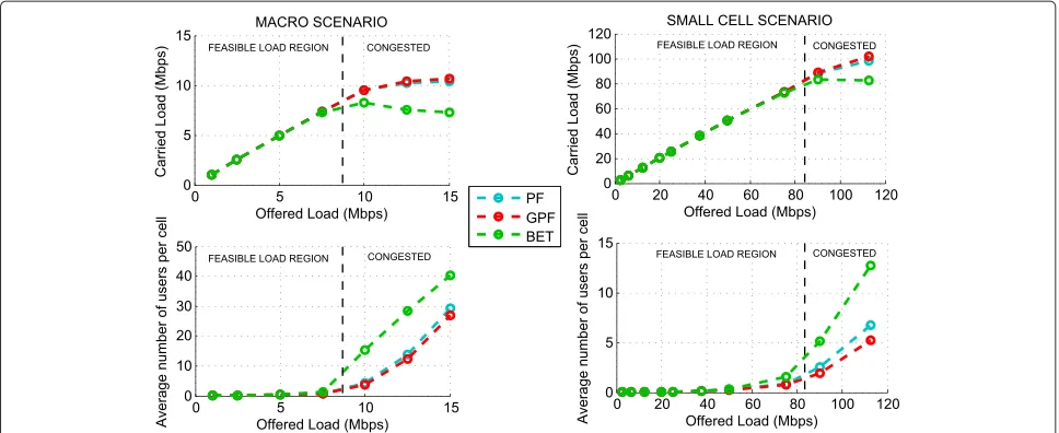
We will begin the analysis by studying the behaviour of the traffic in terms of the different load regions in the macro-cell and small cell scenarios. The carried load and the average number of users per cell as a function of the offered traffic are presented in Figure 3 for the two scenarios and the three schedulers. The carried load plots (upper graphs) present two different segments: the feasible load region in which the carried load increases linearly and matches the offered load, and the congestion region, where the network cannot cope with the amount of demanded traffic. The feasible load region reaches approximately 7.5 Mbps offered load in the macro-only case and 75 Mbps offered load in the small cell case. The evolution of the carried load with increasing traffic is very similar in both scenarios.
Figure 3Scheduler performance comparison. Top: carried load vs. offered load. Bottom: average number of active users per cell over offered load.
of users per cell (bottom part of Figure 3) is kept low in the feasible load region but quickly grows beyond the conges-tion point. As the system is unstable in this region and the results are therefore highly dependent on parameters such as the simulation time, we will focus on the feasible region for the remainder of the article. In line with the results presented in [15] and [20] for the dense small cell case, the scheduling algorithm which provides the best results in terms of these two metrics is GPF, both for the macro-cell and the small cell scenario. The reason is that this sched-uler assigns a higher priority to users under better SINR conditions than PF and BET. These users get served faster and, given the chosen open-loop traffic model, they can leave the network more quickly, reducing the generated interference. This results in an overall performance gain in the network. Therefore, we will only show the statistics obtained under the GPF scheduler in the following figures. The behaviour observed in Figure 3, both for the car-ried load and the number of users per cell, can help us choose a representative offered load value for each of the three characteristic traffic regions. These values and the percentage of active cells in each region are indicated in Table 2. The table serves as a reference for the following
figures in the article, where we will not refer explicitly to the offered load value but to the traffic region.
4.2 Cell occupation statistics
One result from Table 2 that immediately comes to the forefront is the low percentage of active cells in region 3, within the feasible region but close to the conges-tion point. We can examine the situaconges-tion more closely by plotting the empirical cumulative distribution function (cdf ) of the number of users in the cells in this region as shown in Figure 4. The distribution of the users in the cells in both scenarios is very uneven. As previously presented in Table 2, there is a high percentage of inac-tive cells, while some cells contain a fairly large number of users. The majority of the active cells, however, are only simultaneously serving one or two users. Since region 3 is within the feasible region but close to congestion, this behaviour suggests that congestion can be reached without all of the cells being active, as long as some of them are very occupied. Those cells that are very loaded cause such interference to their neighbours that the sys-tem approaches saturation while half of its resources are kept unused. This is the case not only in the dense small
Table 2 Traffic load regions according to offered load and cell occupation
Scenario
Macro cell Small cell
Traffic region Offered load Ave. perc. of Offered load Ave. perc. of
(Mbps) active cells (%) (Mbps) active cells (%)
1 2.5 8.7 25 6.9
2 5 22.8 50 20
Figure 4Cumulative distribution function of the number of active users per cell in traffic load region 3.
cell cluster scenario but also in the macro-cell network, where the cell deployment is regular and the spatial user distribution is uniform. This situation is clearly undesir-able and indicates the need for solutions that can reduce the congestion in the highly loaded cells. As suggested by the performance gains brought by the GPF scheduler, trying to serve the users in a faster way could have a positive impact in terms of reduced interference and cell occupation. Furthermore, inter-cell load balancing solu-tions could be applied to compensate for the uneven use of resources in the network [31].
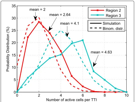
Further insight on the distribution of users within the dense small cell clusters can be attained by studying the probability distribution function (pdf ) of the number of active cells in each TTI. If the occupation of any given cell were statistically independent from the rest, the pdf would follow a binomial distribution [32]. The binomial distribu-tion is the discrete probability distribudistribu-tion of a number of successes,X, achieved aftertindependent trials, each of them having a success probabilityp,
P{X=i} =
t i
pi(1−p)t−i, i=0, 1,. . .,t. (7) Figure 5 presents the empirical distribution of the num-ber of active cells in every TTI for one of the clusters in the dense small cell scenario, together with the theoreti-cal binomial distribution. Region 1 was omitted from the figure as the number of active cells is very low. The values ofpfor the binomial distribution (i.e., the mean probabil-ity that a cell will be active) were obtained from the cdfs of the number of active users per cell, such as the exam-ple presented in Figure 4 (for region 3). The mismatch between the binomial and empirical distributions suggests that there is a coupling between the cells in the cluster
Figure 5Probability distribution function of the number of active cells for one cluster in the dense small cell scenario.
because of mutual interference, and the occupation of the cells is not an independent process.
4.3 Signal and interference levels
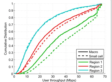
The magnitude of the interference will be quantified in terms of the SINR and DIR of the users. The cdf of the users’ scheduled SINR in the three traffic regions is shown in Figure 6. As expected, the values decrease with increas-ing traffic load as more cells start becomincreas-ing active and the interference increases. Moreover, the SINR is higher for the small cell scenario than for the macro-cell case in regions 1 and 2. This is due to the larger inter-site distance in the macro-only case, making it more probable to have users located far from the serving cell and in lower SINR conditions. On the other hand, the larger number of users in region 3 increases the diversity and hence the values are very similar in both scenarios. The user throughput is directly linked to the SINR and therefore exhibits the same behaviour as the latter with regard to the traffic load regions and network scenarios, as shown in Figure 7.
Figure 6Cumulative distribution function of the user SINR.
due to the higher transmitted power and the lower num-ber of potentially interfering cells compared to the small cell cluster. In general, region 3 is the most interesting one in terms of applying a mechanism to mitigate the strongest interferer, as it is the one providing the largest DIR values, and the potential benefit from mitigation is related to this parameter as shown in (5).
4.4 Time variability of the interference
From the perspective of designing an interference mitiga-tion mechanism, it is important to understand how the interference in the network evolves in time. In order to study this aspect, we present in Figure 9 an example of the time variation of the DIR for 15 of the users. The selected case is the dense small cell scenario at high load (region 3). Each horizontal bar in Figure 9 shows the val-ues of the DIR within the lifetime of one user. The frequent
Figure 7Cumulative distribution function of the user throughput.
Figure 8Cumulative distribution function of the DIR.
colour changes indicate that this value can shift within a few TTIs, sometimes abruptly. It should be noted that our estimation of the DIR does not take into account the fast fading, which does change for every simulated TTI. Therefore, all DIR variations are due to the interference pattern changing when users enter or leave the network. The DIR changes with approximately the same frequency in both scenarios, hence the omission of macro results in Figure 9.
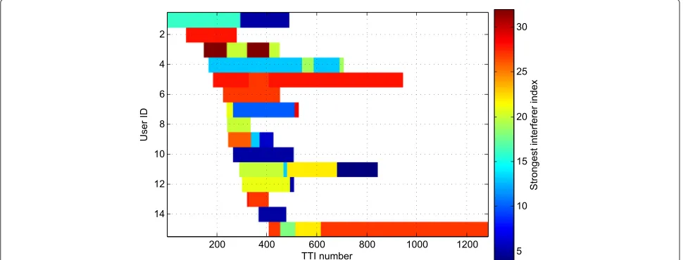
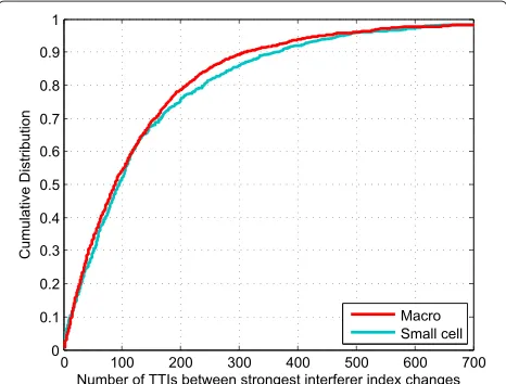
To understand better the source of the DIR changes, Figure 10 shows the time variation of the strongest inter-ferer cell index for the same set of users, in a similar fashion. Looking at Figures 9 and 10, we can see that, while there are frequent shifts in the DIR value, the strongest interferer index remains constant for a longer time. This is true not only for the few users presented in the two figures but also for the rest of the cases, as pictured in Figures 11 and 12, which show the cdf of the number of TTIs between changes in DIR value and in strongest inter-ferer index, respectively. For example, the 50-percentile value is at 7 TTIs between DIR changes but at 100 in the case of the strongest interferer index. This indicates that the changes in the DIR are mainly due to secondary interferers becoming active or inactive.
Figure 9Time evolution of the DIR for 15 of the users. GPF scheduler and 75 Mbps offered load.
achieving more significant gains, and the macro-cell sce-nario starts yielding higher potential benefits. In region 3, there is around a 30% probability of having a throughput gain over 50%, and values as high as 300% can be reached for particular users and TTIs.
5 Discussion of interference mitigation options
The presented results show a comparison of the charac-teristics of the interference in two network scenarios. In spite of the very different nature of the macro-cell and dense small cell cases, the interference behaviour was found to be remarkably similar. Even though previous studies worked under the hypothesis that denser deploy-ments will require the use of custom designed interference mitigation techniques [33], the findings in this article point out that the performance in such cases could be improved by applying similar solutions to those utilized in
macro-cell deployments. Moreover, the gains that could be achieved seem to be comparable.
In general, interference mitigation techniques can be classified in two groups [34]: network-based coordination and user equipment-based solutions. Interference can be mitigated from the network side by limiting the resources in the cells which cause a significant portion of the inter-ference. As explained in [35], there is an important trade-off to consider when applying resource partitioning. On the one hand, there will be a performance increase for the users that were affected by the interference. We can quan-tify this increase as a benefit metric. On the other hand, users served by the cells where resources have been lim-ited will undergo a performance decrease, which can be considered as the cost metric of the solution. As long as the benefit is higher than the cost, the applied technique will bring an overall improvement in the network.
Figure 11Cumulative distribution function of the number of TTIs between changes in DIR value.
In addition to network-based coordination, the user equipment can play a significant role in mitigating the interference by means of advanced receivers, operating in a linear [30,36] or non-linear fashion [37]. The use of advanced receivers presents an inherent advantage in that, since the interference is mitigated at the receiver, there is no need to limit the interfering cell’s resources, effectively eliminating the performance cost that network-based coordination implies. However, user equipment-based techniques are not exempt from limitations. For example, linear advanced receivers withMantennas can only suppress up toM−rsources of interference [38], with rbeing the transmission rank, while non-linear advanced receivers can have stringent SINR requirements of the
Figure 12Cumulative distribution function of the number of TTIs between changes in strongest interferer index.
Figure 13Potential throughput increase with ideal cancellation of the main interferer (%). Scheduling algorithm: GPF.
strongest interference source, to be able to reliably esti-mate, reconstruct and cancel it from the total received signal.
The chosen interference mitigation solution should be dynamic enough to track the changes in the interference profile as suggested by Figures 11 and 12. It is usually more important to curb the effect of the strongest interferer than of the secondary ones, and the strongest interferer index was shown to change with a median period of 100 TTIs. This period is short enough to suggest that some solutions in the literature could be re-evaluated or modified to allow for more dynamic updates. In particu-lar, most of the studies focused on macro-only scenarios have traditionally employed rather static mechanisms (an example is frequency reuse techniques [2]). In a sce-nario with user mobility or with a smaller packet size, the time variability of the interference would increase, further reinforcing the need for more dynamic solutions.
6 Future work
interference more variable and accentuating the need for sufficiently dynamic scheduling and interference mitiga-tion solumitiga-tions.
The findings presented in this paper could be applied to the design of joint inter-cell interference mitigation tech-niques combining some of the discussed options, includ-ing both network-based coordination and receiver-side interference suppression.
7 Conclusions
This article analysed the interference characteristics, per-formance and use of resources in two different LTE-A deployments: a regular macro-cell network and a network comprising dense small cell clusters. These aspects were examined under a dynamic traffic model with different amounts of offered traffic. The two deployments exhib-ited a strikingly similar behaviour in the different traffic load regions: both the performance figures and the time variability of the interference were comparable. The sim-ilarity became more noticeable with increasing offered loads.
The extent to which the main interferer impacts on the user performance was evaluated by means of the dominant interference ratio. This parameter was related through theoretical expressions to the potential benefit from mitigating the strongest source of interference, indi-cating a potential for notable performance gains in both scenarios. Furthermore, since the interference patterns in the two deployments show a strong resemblance, similar interference mitigation solutions could be applied.
Competing interests
The authors declare that they have no competing interests.
Acknowledgements
The authors would like to thank Jens Steiner from Nokia Networks for his helpful contributions to the study.
Author details
1Department of Electronic Systems, Aalborg University, Fredrik Bajers Vej 7, 9220 Aalborg, Denmark.2Nokia Networks, Alfred Nobels Vej 21C, 9220 Aalborg, Denmark.
Received: 29 June 2014 Accepted: 25 March 2015
References
1. H Holma, A Toskala,LTE for UMTS: Evolution to LTE-Advanced, 1st edn. (John Wiley & Sons, Ltd, Chichester, 2006)
2. A Simonsson, inIEEE 65th Vehicular Technology Conference (VTC 2007-Spring). Frequency reuse and intercell interference co-ordination in E-UTRA (IEEE, New York, 2007), pp. 3091–3095
3. E Pateromichelakis, M Shariat, A ul Quddus, R Tafazolli, On the evolution of multi-cell scheduling in 3GPP LTE/LTE-A. IEEE Commun. Surv. Tutorials. 15(2), 701–717 (2013)
4. G Boudreau, J Panicker, N Guo, R Chang, N Wang, S Vrzic, Interference coordination and cancellation for 4G networks. IEEE Commun. Mag. 47(4), 74–81 (2009). doi:10.1109/MCOM.2009.4907410
5. J Lee, Y Kim, H Lee, BL Ng, D Mazzarese, J Liu, W Xiao, Y Zhou, Coordinated multipoint transmission and reception in LTE-advanced systems. IEEE Commun. Mag.50(11), 44–50 (2012). doi:10.1109/MCOM.2012.635368
6. X Wang, B Mondal, E Visotsky, A Ghosh, inIEEE International Conference on Communications Workshops (ICC), 2014. Coordinated scheduling and network architecture for LTE macro and small cell deployments (IEEE, New York, 2014), pp. 604–609
7. A Damnjanovic, J Montojo, Y Wei, T Ji, T Luo, M Vajapeyam, T Yoo, O Song, D Malladi, A survey on 3GPP heterogeneous networks. IEEE Wireless Commun.18(3), 10–21 (2011). doi:10.1109/MWC.2011.587649 8. JG Andrews, Seven ways that HetNets are a cellular paradigm shift. IEEE
Commun. Mag.51(3), 136–144 (2013). doi:10.1109/MCOM.2013.647687 9. KI Pedersen, Y Wang, S Strzyz, F Frederiksen, Enhanced inter-cell
interference coordination in co-channel multi-layer LTE-advanced networks. IEEE Wireless Commun.20(3), 120–127 (2013). doi:10.1109/MWC.2013.654929
10. T Nakamura, S Nagata, A Benjebbour, Y Kishiyama, H Tang, X Shen, N Yang, N Li, Trends in small cell enhancements in LTE advanced. IEEE Commun. Mag.51(2), 98–105 (2013). doi:10.1109/MCOM.2013.646119 11. LGU Garcia, KI Pedersen, PE Mogensen, Autonomous component carrier
selection: interference management in local area environments for LTE-advanced. IEEE Commun. Mag.47(9), 110–116 (2009). doi:10.1109/MCOM.2009.5277463
12. Y Wang, N Marchetti, IZ Kovacs, PE Mogensen, KI Pedersen, TB Sorensen, inIEEE 70th Vehicular Technology Conference (VTC 2009-Fall). An interference aware dynamic spectrum sharing algorithm for local area LTE-Advanced networks (IEEE, New York, 2009), pp. 1–5.
doi:10.1109/VETECF.2009.5379036
13. 3GPP, Small cell enhancements for E-UTRA and E-UTRAN - physical layer aspects (Release 12). TR 36.872 (2013)
14. N Bhushan, J Li, D Malladi, R Gilmore, D Brenner, A Damnjanovic, R Sukhavasi, C Patel, S Geirhofer, Network densification: the dominant theme for wireless evolution into 5G. IEEE Commun. Mag.52(2), 82–89 (2014). doi:10.1109/MCOM.2014.673674
15. V Fernandez-Lopez, KI Pedersen, B Soret, inIEEE 80th Vehicular Technology Conference (VTC 2014-Fall). Effects of interference mitigation and scheduling on dense small cell networks (IEEE, New York, 2014), pp. 1–5 16. HS Jo, YJ Sang, P Xia, JG Andrews, Heterogeneous cellular networks with
flexible cell association: a comprehensive downlink SINR analysis. IEEE Trans. Wireless Commun.11(10), 3484–3495 (2012).
doi:10.1109/TWC.2012.081612.111361
17. A Tukmanov, Z Ding, S Boussakta, A Jamalipour, On the impact of network geometric models on multicell cooperative communication systems. IEEE Wireless Commun.20(1), 75–81 (2013). doi:10.1109/MWC.2013. 647220
18. JG Andrews, RK Ganti, M Haenggi, N Jindal, S Weber, A primer on spatial modeling and analysis in wireless networks. IEEE Commun. Mag.48(11), 156–163 (2010). doi:10.1109/MCOM.2010.562198
19. C Coletti, H Liang, H Nguyen, IZ Kovács, B Vejlgaard, R Irmer, N Scully, in IEEE 76th Vehicular Technology Conference (VTC 2012-Fall). Heterogeneous deployment to neet traffic demand in a realistic LTE urban scenario (IEEE, New York, 2012), pp. 1–5
20. P Ameigeiras, Y Wang, J Navarro-Ortiz, P Mogensen, J Lopez-Soler, Traffic models impact on OFDMA scheduling design. EURASIP J. Wireless Commun. Netw.2012(1), 61 (2012). doi:10.1186/1687-1499-2012-61 21. 3GPP, Technical Specification Group Radio Access Network; Evolved Universal Terrestrial Radio Access (E-UTRA); further advancements for E-UTRA physical layer aspects (Release 9). TR 36.814 (2010) 22. V Paxson, S Floyd, Wide area traffic: the failure of Poisson modeling.
IEEE/ACM Trans. Netw.3(3), 226–244 (1995). doi:10.1109/90.39238 23. F Kelly, Charging and rate control for elastic traffic. Eur. Trans.
Telecommunications.8(1), 33–37 (1997)
24. G Monghal, KI Pedersen, IZ Kovacs, PE Mogensen, inIEEE 67th Vehicular Technology Conference (VTC 2008-Spring). QoS oriented time and frequency domain packet schedulers for the UTRAN Long Term Evolution (IEEE, New York, 2008), pp. 2532–2536
25. K Brueninghaus, D Astely, T Salzer, S Visuri, A Alexiou, S Karger, GA Seraji, inIEEE 16th International Symposium on Personal, Indoor and Mobile Radio Communications (PIMRC 2005). Link performance models for system level simulations of broadband radio access systems, vol. 4 (IEEE, New York, 2005), pp. 2306–23114
27. D Lopez-Perez, I Guvenc, IX Chu, Mobility management challenges in 3GPP heterogeneous networks. IEEE Commun. Mag.50(12), 70–78 (2012). doi:10.1109/MCOM.2012.6384454
28. 3GPP, Technical Specification Group Radio Access Network; Evolved Universal Terrestrial Radio Access (E-UTRA); Physical layer procedures (Release 12). TS 36.213 (2014)
29. IZ Kovacs, M Kuusela, E Virtej, KI Pedersen, inIEEE 67th Vehicular Technology Conference (VTC 2008-Spring). Performance of MIMO aware RRM in downlink OFDMA (IEEE, New York, 2008), pp. 1171–1175 30. FML Tavares, G Berardinelli, NH Mahmood, TB Sorensen, PE Mogensen, in
IEEE 78th Vehicular Technology Conference (VTC 2013-Fall). On the potential of interference rejection combining in B4G networks (IEEE, New York, 2013), pp. 1–5
31. JG Andrews, S Singh, Q Ye, X Lin, HS Dhillon, An overview of load balancing in HetNets: old myths and open problems. IEEE Wireless Commun.21(2), 18–25 (2014). doi:10.1109/MWC.2014.6812287 32. SM Ross,Introduction to Probability and Statistics for Engineers and
Scientists. (John Wiley & Sons, 1987)
33. N Bhushan, J Li, D Malladi, R Gilmore, D Brenner, A Damnjanovic, R Sukhavasi, C Patel, S Geirhofer, Network densification: the dominant theme for wireless evolution into 5G. IEEE Commun. Mag.
52(2), 82–89 (2014)
34. B Soret, KI Pedersen, NTK Jørgensen, V Fernández-López, Interference coordination for dense wireless networks. IEEE Commun. Mag. 53(1), 102–109 (2015). doi:10.1109/MCOM.2015.7010522
35. R Agrawal, A Bedekar, S Kalyanasundaram, N Arulselvan, T Kolding, H Kroener, inIEEE 79th Vehicular Technology Conference (VTC 2014-Spring). Centralized and decentralized coordinated scheduling with muting (IEEE, New York, 2014), pp. 1–5
36. K Pietikainen, F del Carpio, H Maattanen, M Lampinen, T Koivisto, M Enescu, inIEEE 75th Vehicular Technology Conference (VTC 2012-Spring). System-level performance of interference suppression receivers in LTE system (IEEE, New York, 2012), pp. 1–5
37. 3GPP, Technical Specification Group Radio Access Network; Study on Network-Assisted Interference Cancellation and Suppression (NAICS) for LTE (Release 12). TS 36.866 (2013)
38. JH Winters, Optimum combining in digital mobile radio with cochannel interference. IEEE J. Sel. Areas Commun.2(4), 528–539 (1984). doi:10.1109/T-VT.1984.2400
Submit your manuscript to a
journal and benefi t from:
7Convenient online submission 7Rigorous peer review
7Immediate publication on acceptance 7Open access: articles freely available online 7High visibility within the fi eld
7Retaining the copyright to your article