Adaptive CSI and feedback estimation in LTE and beyond: a Gaussian process regression approach

(1)

R E S E A R C H

Open Access

Adaptive CSI and feedback estimation in LTE

and beyond: a Gaussian process regression

approach

Alessandro Chiumento

1,2*

, Mehdi Bennis

3

, Claude Desset

1

, Liesbet Van der Perre

1,2

and Sofie Pollin

1,2

Abstract

The constant increase in wireless handheld devices and the prospect of billions of connected machines has compelled the research community to investigate different technologies which are able to deliver high data rates, lower latency and better reliability and quality of experience to mobile users. One of the problems, usually overlooked by the research community, is that more connected devices require proportionally more signalling overhead.

Particularly, acquiring users’ channel state information is necessary in order for the base station to assign frequency resources. Estimating this channel information with full resolution in frequency and in time is generally impossible, and thus, methods have to be implemented in order to reduce the overhead. In this paper, we propose a channel quality estimation method based on the concept of Gaussian process regression to predict users’ channel states for varying user mobility profiles. Furthermore, we present a dual-control technique to determine which is the most appropriate prediction time for each user in order to keep the packet loss rate below a pre-defined threshold. The proposed method makes use of active learning and the exploration-exploitation paradigm, which allow the controller to choose autonomously the next sampling point in time so that the exploration of the control space is limited while still reaching an optimal performance. Extensive simulation results, carried out in an LTE-A simulator, show that the proposed channel prediction method is able to provide consistent gain, in terms of packet loss rate, for users with low and average mobility, while its efficacy is reduced for high-velocity users. The proposed dual-control technique is then applied, and its impact on the users’ packet loss is analysed in a multicell network with proportional fair and maximum throughput scheduling mechanisms. Remarkably, it is shown that the presented approach allows for a reduction of the overall channel quality signalling by over 90 % while keeping the packet loss below 5 % with maximum throughput schedulers, as well as signalling reduction of 60 % with proportional fair scheduling.

Keywords: 5G; Channel state information; OFDMA; Signalling overhead; LTE; Dual control; Active learning

1 Introduction

Future cellular networks are envisioned to provide extremely high quality of service to an ever increasing number of interconnected users [1]. Many technologies are currently being explored in order to evolve from current 4G networks to future 5G communication. One aspect that has yet to be fully addressed is the signalling overhead imposed on a network with billions of con-nected devices [2–4]. The control information overhead

*Correspondence: [email protected]

1Interuniversity Micro-Electronics Center (IMEC) vzw, Kapeldreef-75, B-3001 Leuven, Belgium

Full list of author information is available at the end of the article

is, in fact, still a very relevant problem for 4G cellu-lar networks, such as long term evolution (LTE). Future 5G networks will, most likely, make use of the same radio access technology utilised by LTE: orthogonal fre-quency division multiple access (OFDMA). In this work, we present techniques to predict and minimise a user’s packet loss by means of limiting the control information in the time domain for a downlink OFDMA network. The simulations are carried out in an LTE environment as this is the most advanced cellular network available today but the methods presented and the results achieved can be easily generalised for future 5G scenarios. In LTE, OFDMA divides the bandwidth into orthogonal blocks, called physical resource blocks (PRBs), and a frequency

(2)

domain scheduler assigns such PRBs to the served users based on their channel conditions [5]. In order to pro-vide each user with the highest quality of service, the base stations employ adaptive modulation and coding (AMC) techniques which adjust different modulation and cod-ing schemes (MCS) used for transmission accordcod-ing to the channel state information (CSI) signals fed back from the users. Therefore, relevant and timely CSI signalling is extremely important to allocate the wireless resources to the users and maximise the overall network capacity. Full CSI feedback (FB), although optimal in maximising the downlink capacity, cannot be used in LTE as the standard quantises both the amount of channel state information the users feed back in the frequency domain as well as how often this information can be reported in time [6].

In [7], we have shown that it is possible to limit chan-nel state information, in frequency, without loss in per-formance if the freed uplink bandwidth is allocated for payload communication. We have also shown that the number of served users under different fairness strategies, imposed by the frequency resource allocation mecha-nisms, influence the impact of FB allocation strategies and that it is possible to determine the optimal FB allocation. The impact of FB information is then a function of the number of users served by the base station, their channel quality and the scheduling algorithm used to assign the PRBs. In this work, we show that it is possible to compen-sate for the capacity loss due to reducing the CSI signalling in time, even with already quantised frequency resolution, via the usage of per-user channel quality prediction and per-user dynamic assignment of prediction time windows. Considerable work has been devoted by the research community to either channel quality prediction or feed-back overhead reduction. In [8], the authors implement and compare various signal-to-interference-and-noise ratio (SINR) prediction algorithms and conclude that high gains can be expected when using covariance-based pre-dictors for low mobility users. In [9], the authors present a prediction method used to compensate for CSI delay. The estimation is performed at the mobile user side and the predictor takes into account the Doppler shift of each user for more accurate estimation. Both works make use of the users’ Doppler shift to determine the time duration of the channel quality estimation; this procedure, although well established, might lead to erroneous predictions, a negative correlation is generally present between predic-tion quality and Doppler shift. On the other hand, a high mobility user might witness a better, less variable chan-nel than a low mobility user. Furthermore, users have to predict the SINR themselves, depleting their battery life. In [10], the authors propose a dynamic Channel Qual-ity Index (CQI) allocation method, which is a quantised value indicative of the SINR experienced by the users and predicted at the base station. The CQI allocation time of

each user is adapted based on the instantaneous packet loss of each user. In [11], the same authors expand their results by including CQI prediction at the base station. They use a linear predictor and compensate for errors by reducing or increasing the prediction windows based on the users’ packet loss. In [12], the authors present a non-predictive signalling reduction scheme where only users with low SINR are allowed to feed back expensive instan-taneous CQI information while high SINR users only transmit wideband information. Even though the method decreases the signalling information, it is carried out for a limited and fixed time window (2 ms) and a single cell scenario, ignoring the underlying network dynamics due to interference, traffic load, etc.

The main objectives of this work are twofold. Firstly, we propose an online and adaptive CQI prediction scheme to estimate users’ channel quality variations at the base station side, while compensating for some of the quantiza-tion noise introduced by sampling the SINR at certain CQI values. The proposed CSI estimation approach is based on Gaussian process regression which has been shown to be efficient in the presence of noisy measurements [13]. Gaussian processes (GPs) are also used to estimate the distribution of variables rather than their values, making them attractive for solid predictions over noisy datasets. Furthermore, GPs provide a principled framework in which their parameters can be estimated with maximum likelihood techniques removing constraints related to the fine-tuning of such predictors [14].

Secondly, we leverage the GP-based prediction mech-anism for the CQI assignment problem, in which a base station controller is able to monitor the behaviour of each served user and assign a personalised prediction time window based on that user’s performance and require-ments. For this procedure, a dual-control system based on active learning, as introduced in [15], is used. The dual controller is able to monitor and predict the base station’s performance and assign a time window to each user based on specific requirements. The active learning component is used to limit the amount of necessary data sampling before an optimal policy is reached. In order to demonstrate the effectiveness of the proposed methods, we consider a multi-user, multi-cell LTE network. The quality of the GPR for CQI prediction is presented for dif-ferent user speeds, and afterwards, simulation results for the dual-control system are shown for both proportional fair and maximum throughput scheduling.

(3)

dynamically the optimal prediction window for a given user. In Section 5, the performance of the proposed solu-tions is presented. Finally, in Section 6, the concluding remarks are drawn.

2 System model

2.1 Network model

The network is composed ofBbase stations (eNBs), each serving an equal amountNU of mobile users (MUs). LTE makes use of time-frequency resource allocation, in which the frequency bandwidth is split into orthogonal units called physical resource blocks, each of which is allocated separately. For each PRBk an MU measures its received SINR, defined as:

wherePiandGiare the transmit power and transmission gains of the serving base stationiwhilePjandGjare the transmit power and transmission gains of the interfering base stationsjandnkis the additive Gaussian noise.

Even though the PRB is the smallest unit, the base sta-tion can allocate to each user; in order to limit the amount of signalling information, each MU is unable to feed back detailed information on each PRB, and thus the PRBs are generally grouped in subbands and only one value for such band is measured. This value is referred to as the effective SINR and is computed with the Effective Exponential SNR Mapping (EESM) formulation [16]:

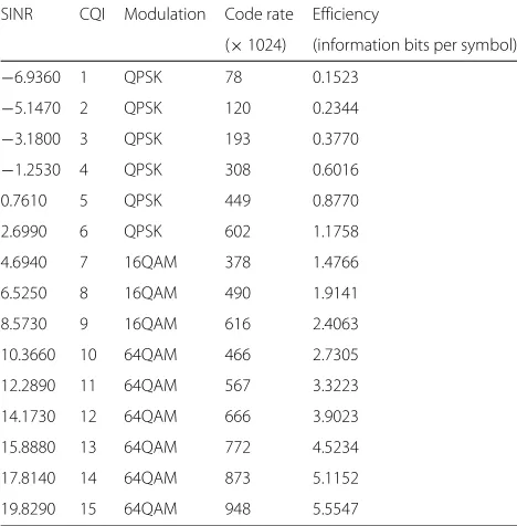
where S represents the size of the subband and λ is a parameter empirically calibrated by the base station. The effective SINR is then quantised into a channel quality indicator (CQI) value, indicative of the highest modula-tion and code rate the base stamodula-tion may use while keeping a packet error rate (PER) below a target of 10 % as shown in Table 1 [17]. Each user then feeds back these CQI values to the base station.

Once the eNB has collected the CQIs for the entire bandwidth, it schedules resources for each user according to its resource allocation function.

2.2 LTE feedback schemes

2.2.1 “Frequency domain feedback”

In a practical scenario, the CQI reporting is not per-formed for each PRB but it is quantised in frequency to reduce the control signalling overhead. The three report-ing techniques used in the LTE standard are presented in [6].

• Wideband : each user transmits a single 4-bit CQI value for all the PRBs in the bandwidth.

Table 1SINR and CQI mapping to modulation and coding rate

SINR CQI Modulation Code rate Efficiency

(×1024) (information bits per symbol)

−6.9360 1 QPSK 78 0.1523

−5.1470 2 QPSK 120 0.2344

−3.1800 3 QPSK 193 0.3770

−1.2530 4 QPSK 308 0.6016

0.7610 5 QPSK 449 0.8770

2.6990 6 QPSK 602 1.1758

4.6940 7 16QAM 378 1.4766

6.5250 8 16QAM 490 1.9141

8.5730 9 16QAM 616 2.4063

10.3660 10 64QAM 466 2.7305

12.2890 11 64QAM 567 3.3223

14.1730 12 64QAM 666 3.9023

15.8880 13 64QAM 772 4.5234

17.8140 14 64QAM 873 5.1152

19.8290 15 64QAM 948 5.5547

• Higher Layer configured or subband level : the bandwidth is divided intoqsubbands ofSconsecutive PRBs and each user feeds back to the base station a 4-bit wideband CQI and a 2-4-bit differential CQI for each

subband. The value ofkis bandwidth dependent and

is given in Table 2, whereN_PRBDL is the total number of downlink PRBs in the bandwidth (table 7.2.1-2 in [6]).

• User-selected, or Best-M : each user selectsM

preferred subbands of equal sizeSand transmits to the base station one 4-bit wideband CQI and a single 2-bit CQI value that reflects the channel quality over the selectedMsubbands. Additionally, the user reports the position of the selected subbands using

PFBbits, wherePFB, as given in [6], is:

(4)

whereNPRBDL

M

is the binomial coefficient. The value of

Mand the amount of PRBs in each subband are given

in Table 3 (table 7.2.1-5 in [6]):

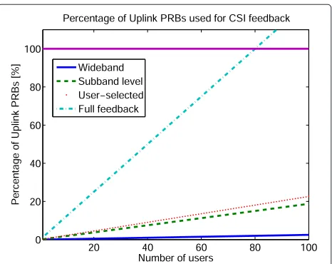
Amongst the three standard compliant feedback schemes, only the subband level technique allows the base station to investigate the channel quality of the complete bandwidth with equal amount of detail between sub-bands. For this reason, it has been chosen, in this work, as the preferred FB method and the GPR process is aided by the constant resolution over the bandwidth. Further-more, excluding the wideband FB, which does not allow frequency selective scheduling, it is the least expensive in terms of uplink bandwidth, Table 4 includes the mathe-matical definitions of the bit cost of the different feedback allocation methods presented in Section 2 when the stan-dard code rate of 1₂ is used. Figure 1 shows the amount of feedback required for the different schemes as a func-tion of the number of users with a 20 MHz (100 PRBs) UL bandwidth using QPSK modulation (the horizontal line represents the total uplink bandwidth).

2.2.2 “Time domain feedback”

The CSI is limited in the time domain. The periodicity of CQI reporting is determined by the base station, and the CQI signalling is divided into periodic and aperiodic reporting [18]. In case of aperiodic CQI signalling, the eNB specifically instructs each user on which frequency granularity to use and when the reporting has to occur. With aperiodic reporting, the eNB can make use of any of the CQI standard compliant feedback methods dis-cussed above. Periodic CQI reporting, on the other hand, is more limited and only wideband and user-selected feed-back methods can be used. In this case, the CQI messages are transmitted to the base station with constant period-icity, e.g. in case of periodic wideband feedback in an FDD system, each user can report its CQI values every 2, 5, 10, 16, 20, 32, 40, 64, 80 and 160 ms. For the remainder of this work, we assume that an aperiodic feedback is used, as this allows the eNB controller to adapt the CQI transmission time more freely than with periodic reporting.

Table 3Subband size (S) and number of subbands (M) vs. system bandwidth for user-selected feedback

System bandwidth Subband size M

NDL

PRB (S)

6–7 NA NA

8–10 2 1

11–26 2 3

27–63 3 5

64–110 4 6

Table 4Bit cost of the frequency selective standard complaint FB methods

Feedback scheme Bit cost

Wideband 2·(4·NU)

Subband level 2·(4+2·q)·NU

User-selected 2·(4+2+ log2N

DL PRB M

)·NU

2.3 Resource allocation mechanisms

While the CQI information defines the achievable rate on each PRB, the overall cell transmission rate is a func-tion of the resource allocafunc-tion mechanism implemented at the base station. Two scheduling methods are used in this work to define the impact of CQI prediction and assignment on the cell throughput:

• Best CQI (BCQI), or max-rate, is a greedy scheduler

designed to maximise the cell throughput. For each PRB, only the user with the highest channel quality indicator is scheduled.

• Proportional Fair (PF): this scheduler is designed to aim for high throughput while maintaining fairness amongst users. PF schedules users when they are at their peak rates relative to their own average rates, at a given time instantt, PF schedules user

xi=arg maxr_Ri,_ik₍(_tt₎), whereri,k(t)is the instantaneous

data rate of userxion PRBkat timetandRi(t)is the

average throughput, computed with moving time windowT, such thatRi(t)= _T1tj=t−Tri(j).

3 CQI prediction

We now turn our attention to the description of the CQI estimation methods. The estimation process is carried out

(5)

to compensate for the reduction in CQI reporting in time. Given the relationship between CQI and SINR described in Section 2.1, predicting the CQI is equivalent to predict-ing a noisy function of the relative effective SINR. Due to the Gaussian nature of the SINR distribution and the inherent flexibility of Gaussian Processes for regression, these have been selected in this work.

3.1 Gaussian process regression

The objective of GPR is to estimate a function f in an online manner with low complexity. A Gaussian process (GP) is defined as a probability distribution over some variables, where any finite subset of these variables forms a joint Gaussian distribution [19]. This means that, instead of making assumptions on the elements of a dataset, a GP infers their distribution. Let us consider a datasetD =

xi, ,yi

with i = 1, 2,. . .n, where eachxi andyi repre-sent the input and output points. We define the relation between such vectors asy= f(x)+n, wherenis a zero-mean Gaussian noise with varianceσ2_{. A GP is defined as}

a collection of random variables, such that any finite set has a joint Gaussian distribution. Since a Gaussian distri-bution is completely defined by its mean and covariance matrix, a GP is completely defined by its mean function m(x)and covariance functionk(x,x˜), expressed as:

f(x)∼GP(m(x),k(x,x˜)), (4)

where

m(x) = E[f(x)]

k(x,x˜) = E[(f(x)−m(x))(f(x˜)−m(˜x))] . (5)

The output can be defined by a GP, such that:

y∼GP(m(x),k(x,x˜)+σ2I), (6)

By aggregating the inputs into a vectorX and the out-puts into a vectorY, the GP estimates the value ofyˆat a future pointx∗, assuming a multi-variate distribution:

whereK(X,X)is the matrix representation of the covari-ance functions of the input samples and K(X,x∗) is the covariance matrix of the overall input dataset andk(x∗,x∗) is the autocorrelation of the future data point. The poste-rior probabilityyˆ|Yis given by [13]:

ˆ

y|Y ∼NK(X,x∗)K(X,X)+σ_n2I−1Y, k(x∗,x∗)

−K(X,x_∗)K(X,X)+σ_n2I−1K(X,x_∗)T, (8)

The best estimate for yˆ is given by the mean of such distributionm(Yˆ) = K(X,x∗)K(X,X)+σ_n2I−1Y

and the variance Var(Yˆ) = k(x∗,x∗) − K(X,x∗)

K(X,X)+σ_n2I−1K(X,x∗)T represents the uncertainty of the current estimate. The GP is then fully defined by its covariance and mean functions and their parameters.

3.2 Covariance function selection

In order to obtain a good estimate of the future measure and its underlying distribution, a covariance function that best fits the nature of the system has to be selected. As the mean can easily be set to zero if some pre-processing is carried out, it is usually ignored [13]. Although the covariance functionKis limited to positive semi-definite functions, many choices are present in literature able to fit to dynamic, time-varying systems [19]. The most impor-tant feature when choosing a covariance function is its smoothness, i.e. how much the value of the function sam-pled at a point x∗ correlates with the same function at points close tox∗. A function that presents high smooth-ness might not be representative of a fast-varying system. It could be possible, in theory, to observe a large reali-sation of an input dataset and generate a specific covari-ance function which models the witnessed behaviour very closely. This is normally not performed as a few families of covariance functions are present in literature which adapt quite well to a large selection of problems in which the data can be modelled as a multivariate Gaussian distribu-tion [13]. For this reason, in the current task of modelling, the channel quality for users with varying mobility a Matérn class covariance function has been selected [20]:

k(x,x_∗)=h22

(6)

Fig. 2Dual control with active learning framework. Block diagram of the proposed dual control with an active learning method

over the product of the prior and the likelihood function. Since both are Gaussian, the marginal likelihood is also Gaussian and is expressed in analytical form:

pY|X,θ,σ2=

p(Y|f,X,θ,σ2)p(f|X,θ)df

=

N(f,σ2,I)N(0,K)df

= 1

(2π)n2|_K+σ2_I|12

exp

−1 2y

T_K₊_σ2_I−1_y

(10)

Whereθis the set of hyperparameters. Generally speak-ing, for simplicity, the log marginal likelihood is max-imised [13]:

logp(Y|X,θ)= −1 2Y

T₍_K₊_σ2 nI)−1Y

−1

2log|K+σ

2 nI| −

n

2log 2π. (11) By using any multivariate optimization algorithm, the set of hyperparametersθ can be estimated analytically. After the optimization process has reached the analytical solu-tion, the numerical values of the hyperparameters are simply obtained by using the measured input and out-put signals. This is a great advantage over other types of regression as it allows the system to evolve without pre-specifying the parameters and thus limiting the range of estimations [22].

3.3 GPR for CQI prediction

In this work, the eNB makes use of GPR to predict the CQIs values for every subband seen by each user. In order

to make realistic predictions, the output vectorY is used to train the GP. For each user, the base station receives the CQI information for the complete bandwidth, using the subband-level FB quantization scheme discussed in Section 2.2 everytsamp=2ms. The value of the sampling windowtsampis chosen as the minimum allowed by LTE standard to acquire a high number of samples in a short time [23]. After the observation time elapses, say at instant t0, the eNB uses GPR to predict the future CQI values in

each subband as shown in Algorithm 1.

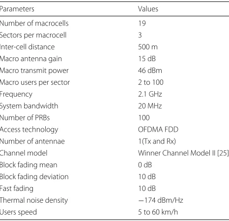
Table 5System parameters

Parameters Values

Number of macrocells 19

Sectors per macrocell 3

Inter-cell distance 500 m

Macro antenna gain 15 dB

Macro transmit power 46 dBm

Macro users per sector 2 to 100

Frequency 2.1 GHz

System bandwidth 20 MHz

Number of PRBs 100

Access technology OFDMA FDD

Number of antennae 1(Tx and Rx)

Channel model Winner Channel Model II [25]

Block fading mean 0 dB

Block fading deviation 10 dB

Fast fading 10 dB

Thermal noise density −174 dBm/Hz

(7)

Algorithm 1:CQI estimation with GPR 1: foreach userudo

2: foreach subbands∈qdo

3: Initialization:Input vectorcqisamp, Output vectorcqipred, Covariance functionK, Noise levelσ, Prediction windowtw

4: whilet<t0do

5: Build historical dataset

cqihist(t)=cqisamp(t).

6: end while

7: whilet≥t0do

8: ift=twthen

9: (1) The GP is trained with the vectorcqihist. 10: (2) The hyperparameters are found by

maximising the log-likelihood (11) 11: (3) The predicted CQIs vectorcqipredof

lengthtwis generated.

12: (4) The base station usescqipredto allocate the users for the nexttwintervals

13: else

14: Update the input dataset with the new sampled valuecqihist(t)=cqisamp(t)

15: end if

16: end while

17: end for

18: end for

4 Dynamic time window optimisation

In this section, we introduce a control mechanism to determine the appropriate duration of the CQI predic-tion window so that the eNB can maintain each user’s

performance within a specified loss margin. Firstly, the dual-control system based on active learning is introduced and, secondly, its implementation in an LTE base station for time windows optimisation is presented.

4.1 Dual control with active learning

A dual-control agent is tasked with controlling a sys-tem based on the current knowledge of its behaviour and to perturb it in order to minimise the uncertainty and make better predictions. By their nature, these objec-tives are conflicting. In this work, we follow the adaptive dual-control method proposed in [15], which provides a solution to the control problem while also limiting the amount of overhead.

Let us define a dynamic, non-linear, partially observable d-dimensional system described by:

yj(t+1)=hj(y(t),c(t))+n(t) with j=1· · ·d, (12)

whereyj(t+1)is the value of the output system at time t + 1, which is function of the system behaviour h(·) given the past observationy(t)and the control function c(t). n(t) is a zero-mean Gaussian noise. In this con-text,h(·)corresponds to the function to be estimated(f), according to the formalism of the previous section. Given a d-dimensional reference signal r(t), the dual-control problem consists in finding the best control strategyμ(t) such that

μ(t)=arg min c(t)

y(t)−r(t), ∀t (13)

(8)

Furthermore, it is possible to limit the amount of data collected by the controller by maximising the informa-tion collected. Ifhˆis an estimate of the system dynamics hbased on previous observations, the dual control with active learning problem consists in finding the optimal strategyμ(t)solving the following optimisation problem:

max

u(t) I(h,ˆ c(t))≈arg minc(t) Var(h,ˆ c(t)) (14)

where I represents the Shannon information of the dynamic system andVaris the variance [15]. The objec-tives of the active dual controller consist in partially iden-tifying the dynamics of the system so that it can be kept as close as possible to the reference signal while sampling only in the points that minimise uncertainty for future predictions. Figure 2 presents a block description of the dual-control framework.

The dual control with active learning can be formally described as (Proposition 4 in [15]): Let the input-output relationship of a discrete-time dynamic system be defined as in Equation 12.

Let hˆ be the predicted estimate of the system’s behaviour, in this case, the packet loss due to reducing the time sampling of CQI values. The predicted future value ˆ

y(t+1)can be inferred as:

ˆ

y(t+1)= ˆh(y(t),c(t))+n(t). (15)

The optimal strategyμis then defined as

μ(t)=arg min c(t) wa

y_ˆ(t+1)−r(t)−weVar(yˆ(t+1),c(t))

(16)

where wa and we represent the action and exploration weights to steer the controller towards either steepest descent to the closest optimal solution (we = 0) or

Fig. 4Packet loss for user moving at 5 km/h over time sampling intervals. This figure shows the packet loss experienced by a user moving at 5 km/h when GPR prediction or CQI averaging are used

Fig. 5Packet loss for user moving at 10 km/h over time sampling intervals. This figure shows the packet loss experienced by a user moving at 10 km/h when GPR prediction or CQI averaging are used

to a complete exploratory behaviour (wa = 0). Gener-ally, the weights can be adjusted so that the controller behaves more exploratory at the beginning of the learn-ing procedure and then moves to a more active controlllearn-ing role.

4.2 Dual control for signalling reduction

In the dual-control framework for dynamic time window optimisation, we make use of the same GPR used for CQI prediction. In this case, the GPR is used to predict the packet losses each user incurs when different time windows are chosen. At time t0, the eNB receives the

CQI FB from each user u, then it chooses a time pre-diction windowtwu(t0)and uses GPR to predict the CQI behaviour for the duration of such window. At the same

(9)

Fig. 7Estimated and real CQI values. The figure shows the actual measured and the predicted CQI values for a user moving at 10 km/h

time, it uses GPR to predict the packet loss Lˆu(t0 +

1,twu(t0))the user will experience given the current time window. The objective of the controller is then to solve, for every useru:

twu(t+1)=arg minwa,uLˆu(t+1)−ru,th

−we,uVar(Lˆu(t+1),twu(t)),

(17)

whereru,this the reference packet loss for useru. At time t0+twu(t0), the eNB measures the actual packet loss suf-fered by the user. The controller then corrects the CQI prediction window accordingly to provide better predic-tions and the process is repeated. Algorithm 2 provides a concise view of the solution above.

Algorithm 2: Dual control with active learning for dynamic CQI FB assignment

1: foreach userudo

2: Initialization:GP hyperparameters, objective weights [wa,we], reference signalru,th

3: whilet>t0do

4: (1) Receive CQI FB from user and estimate the CQI behaviour using GPR.

5: (2) Estimate the system dynamicsLˆusing GPR. 6: (3) Determine the best time windowtw(t+1)by

solving (17) and crop CQI prediction at selected time windowtw(t+1).

7: (4) Schedule the user for the duration of the time windowtw(t+1).

8: (4) Compute the varianceVar(L,tw).

9: (5) Update the dataset with the newly observed pointL(t).

10: end while

11: end for

0 100 200 300 400 500

0.6 0.7 0.8 0.9 1 1.1 1.2 1.3 1.4 1.5

RMSE of CQI prediction over observation window

Training window [ms]

RMSE

0 100 200 300 400

1.7 1.8 1.9 2 2.1 2.2

RMSE

0 100 200 300 400 500

1.3 1.4 1.5 1.6 1.7 1.8 1.9 2

b

c

a

RMSE

(10)

Cosine Matern 1 Matern 3 Matern 5 Neural Network Polynomial RQ 1.7

1.75 1.8 1.85 1.9 1.95 2 2.05 2.1 2.15

RMSE

RMSE for various covariance functions

Fig. 9RMSE of different covariance functions. Comparison of the error committed when different covariance functions are used for the GPR

5 Results

In this section, we will first define the simulation envi-ronment and then provide the results for the proposed models.

5.1 Simulation parameters

The system has been simulated using the open source VIENNA system level simulator [24]. An urban multi-cell environment has been considered to include the effects of multipath propagation and interference; 19 LTE macro-cells are simulated with 30 users per cell, in which only the users in the most central cell are studied to reduce border effects. In order to model the effects of user mobility in a city-like environment, the users have an average speed of 5, 10 or 60 km/h. The propagation model is determinis-tic and based on the Winner Channel Model II [25]. The simulation parameters are included in Table 5.

5.2 Simulation results

Firstly, we present the impact that the various frequency sampling schemes of Section 2.2 have on the packet loss

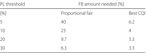
Table 6Percentage FB necessary with dual control

PL threshold FB amount needed [%]

[%] Proportional fair Best CQI

5 40 6.2

10 23 4

20 9.7 3.3

30 6.3 3.3

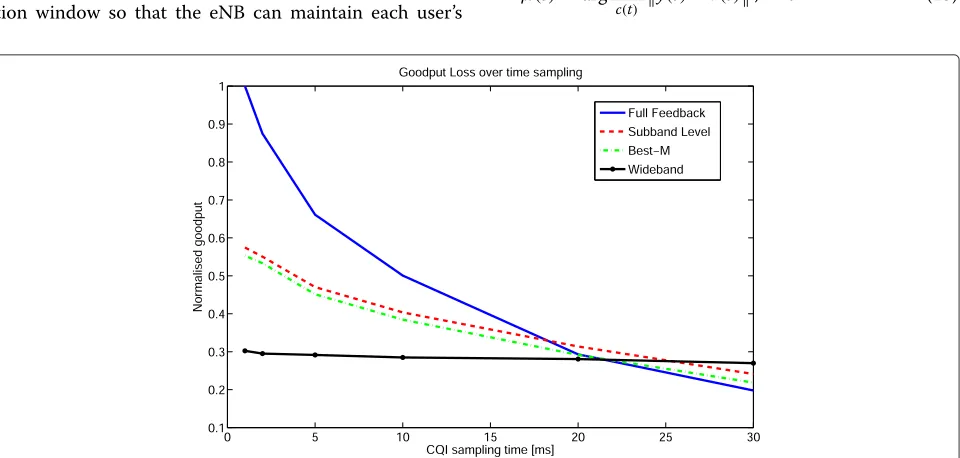
experienced by users. The CQI FB messages are sampled at specific moments in time, and the previously sampled value is used until the next sampling moment. Figure 3 shows the normalised goodput of a user moving at 10 km/h when the full feedback, subband-level, best-M and wideband schemes are employed.

It is visible that there is a loss in goodput when either the CSI frequency sampling methods are used or the CSI sampling time interval is increased. On the other hand, the effects of increasing the duration between sampling instants are less pronounced when the CQI information is quantised in frequency. This is particularly visible for the wideband FB scheme, where the initial goodput is just above one third of the full feedback but the loss in time is almost null. For large time sampling intervals, the three standard compliant FB schemes behave better than the full feedback. For the remainder of this work, the subband level method is employed, as it presents, for almost all the sampling delays considered, the highest gain amongst the standard compliant schemes.

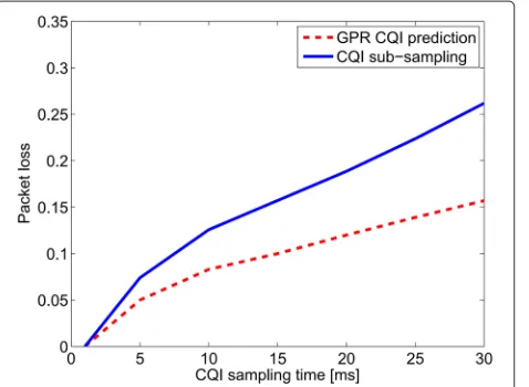
The effects of GPR CQI prediction for fixed CQI time sampling are presented in Figs. 4, 5 and 6 for users with speeds of 5, 10 and 60 km/h. The figures show the aver-age packet loss seen by a user when either prediction or fixed time sampling is used. By fixed sampling, we intend that the base station only uses the last received CQI value until a new one is sampled. For the first two plots, the GPR CQI prediction shows considerable gains over the alternative.

(11)

0 5 10 15 20 25 30 0

0.05 0.1 0.15 0.2 0.25 0.3 0.35 0.4 0.45

Predicted PL for single user

time window duration [ms]

Packet Loss

Predicted behaviour Average sampled value Measured values

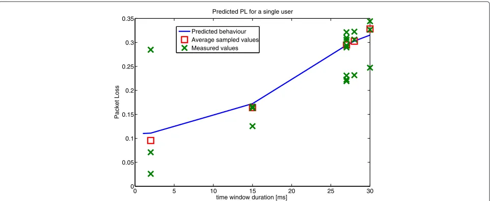
Fig. 10Predicted packet loss and measurements for different prediction time windows. This figure shows the predicted and measured packet loss for various time windows. The figure also shows the final action taken by the controller in order to keep the packet loss below a 10 % threshold

duration. This is due to the fact that the fast varying chan-nel does not allow for reliable estimation for extended time intervals. Nonetheless, it is possible to exploit the GPR estimation’s gain over the sampling if short time windows are used.

Figure 7 shows an example of the estimated and real CQI values for a user moving at 10 km/h with a predic-tion window of 10 ms. There is good accordance between the predicted CQIs and the real values. The GPR is able to model the changes in the user’s channel.

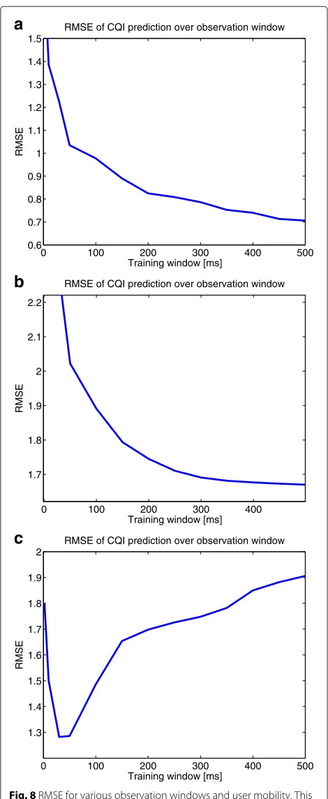
Figure 8 shows the root mean square error (RMSE) of the GPR predictions for different training datasets. In case of users moving at 5 and 10 km/h, we can see that conver-gence is reached and a large observation window allows the GPR to make an accurate estimation. When users have high mobility, on the other hand, a large training can lead to more errors as the time correlation of the CQI values decreases as seen in Fig. 8c.

The impact of different covariance functions on the CQI estimation process with GPR is presented in Fig. 9. The Matérn function with smoothnessv= 3₂behaves best. A detailed analysis of the various functions in the figure can be found in [13].

By using the dual-control scheme, it is possible to set a maximum limit to the user’s packet loss due to lim-ited time feedback. If a user is selected to be scheduled by the eNB, then a predicted packet loss can be inferred with the proposed model and a decision is made based on Equation 17. In order to analyse a dynamic scenario, users with diverse requirements are simulated together; a total of 60 users are served within the cell, of which 30 have low mobility (5 km/h), 20 have average mobility (10 km/h) and 10 are high speed users (60 km/h). Table 6

1 2 3 4 5

0 0.05 0.1 0.15 0.2 0.25 0.3 0.35

RMSE of the prediction at each iteration

a

iterations

RMSE

1 2 3 4 5

0 0.02 0.04 0.06 0.08 0.1 0.12 0.14 0.16

Variance of the predicted model

b

Iterations

Variance

(12)

0 5 10 15 20 25 30 0

0.1 0.2 0.3 0.4 0.5 0.6 0.7

Predicted PL for a single user

Packet Loss

Predicted behaviour Average sampled value Measured values

Fig. 12Predicted packet loss and measurements for different prediction time windows. This figure presents the predicted and measured packet loss for various time windows for a user with bad channel conditions. The figure shows the final action taken by the controller in order to keep the packet loss below a 5 % threshold

shows the percentage of FB required by the system for various packet loss threshold values for both the propor-tional fair and best CQI schedulers after the model has converged to the optimal decision compared to the state of the art where no prediction is used and the CSI is sam-pled every 2 ms. There are considerable gains for both schedulers but, as the PF maximises fairness, every user will be scheduled in the upcoming time slots and thus the time windows have to be inferred so that the predicted packet loss is minimised. On the other hand, since the dual-control model has as input the packet loss of each user, if such user is not scheduled, then the loss is null and a higher time window can be selected. For this reason the best CQI scheduler allows for much higher gains with an almost 94 % reduction in FB signalling when the allowed packet loss is contained to only 5 %.

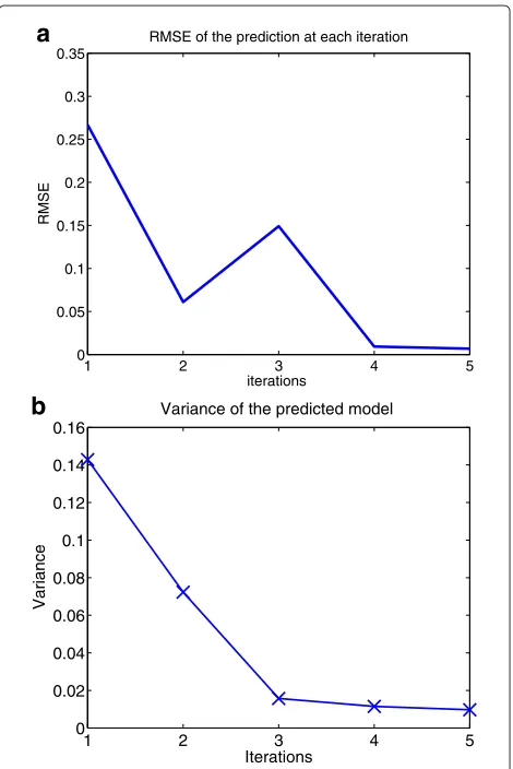
Figure 10 presents the behaviour of the proposed dual-control method in Algorithm 2 for a single user. The packet loss at the sampling instants is indicated with the X markers while the square markers indicate the average sampled packet loss. The proposed solution then grad-ually builds a predicted packet loss behaviour, indicated in Fig. 10 by the continuous curve. At each iteration, the model selects the next time window according to (17) with weights wa = 1 and we = 10 and predicts the packet loss behaviour for the duration of the selected window. After the time window has passed, the eNB samples the packet loss again, corrects its prediction and determines the next prediction time window until it converges to the desired packet loss threshold. In this specific realisation, the packet loss threshold is imposed at 10 % and the opti-mal inferred time window is 5 ms. It is important to notice that, because of the time varying nature of the channel,

1 2 3 4 5 6 7

0 0.1 0.2 0.3 0.4 0.5 0.6 0.7

a

iterations

RMSE

1 2 3 4 5 6 7

0.01 0.015 0.02 0.025 0.03 0.035 0.04 0.045

b

iterations

Variance

(13)

0 5 10 15 20 25 30 0

0.05 0.1 0.15 0.2 0.25 0.3 0.35

Predicted PL for a single user

Packet Loss

Predicted behaviour Average sampled values Measured values

Fig. 14Predicted packet loss and measurements for different prediction time windows. This figure shows the predicted and measured packet loss as function of time prediction windows for a user with very good channel conditions. The final time window chosen by the controller to keep the packet loss below the 30 % threshold is shown in the figure

the measured loss can oscillate even if the time windows’ sampling is kept constant. The GPR takes this into account as measurement noise and is still able to approximate the system dynamics.

Figure 11a, b shows the prediction error calculated at each iteration and the variance of the prediction model; in both cases, the proposed approach reaches the desired behaviour after only five iterations.

In Fig. 12, the packet loss threshold is 5 %. In this case, the base station has to choose a very small prediction win-dow of 2 ms for a high mobility user with high packet loss.

Figure 13a, b shows the prediction error computed at each iteration and the variance of the prediction model. As in the previous case, convergence is attained after five iterations.

The proposed model’s behaviour in case of a low mobil-ity user with good channel is presented in Fig. 14 where the packet loss threshold is imposed at 30 %. In this case, the base station can choose a large prediction window of 27 ms.

Figure 15a, b shows the prediction error committed at each iteration and the variance of the prediction model. In this case, convergence is attained after three iterations.

6 Conclusions

In this work, we have shown that the feedback overhead cannot be overlooked as the number of connected devices keeps increasing. Some solutions are implemented in the frequency domain to limit the impact of this signalling information on the uplink bandwidth but additional restrictions in the time domain are also necessary. We presented a GPR technique to predict the users’ channel

1 2 3 4 5 6 7

0 0.05 0.1 0.15 0.2 0.25

iterations

RMSE

1 2 3 4 5 6 7

0.011 0.012 0.013 0.014 0.015 0.016 0.017 0.018 0.019 0.02

a

b

iterations

Variance

(14)

quality for various speeds limiting the loss incurred by increasing the time sampling period. The proposed CQI prediction method is able to estimate a user’s channel with good accuracy. Furthermore, we have presented a dual-control method based on active learning, able to determine the optimal prediction window given a packet loss threshold. The same method is also able to probe the system in such a way that an optimal solution is reached while also limiting the system’s exploration by maximis-ing the impact of the information collected. The proposed method shows gains of up to 94 % in signalling reduction if best CQI scheduler is used when compared with state of the art if the packet loss is capped to 5 %.

Competing interests

The authors declare that they have no competing interests.

Author details

1_{Interuniversity Micro-Electronics Center (IMEC) vzw, Kapeldreef-75, B-3001}

Leuven, Belgium.2Department of Electrical Engineering (ESAT) KU Leuven, Kasteelpark Arenberg 10, B-3001 Leuven, Belgium.3_{Centre for Wireless} Communications, University of Oulu, 90570 Oulu, Finland.

Received: 20 December 2014 Accepted: 14 May 2015

References

1. R Baldemair, E Dahlman, G Fodor, G Mildh, S Parkvall, Y Selen, H Tullberg, K Balachandran, Evolving wireless communications: addressing the challenges and expectations of the future. Vehicular Technol. Mag. IEEE.

8(1), 24–30 (2013). doi:10.1109/MVT.2012.2234051

2. A Imran, A Zoha, Challenges in k5G: how to empower SON with big data for enabling 5G. Network IEEE.28(6), 27–33 (2014).

doi:10.1109/MNET.2014.6963801

3. E Lähetkangas, K Pajukoski, J Vihriälä, G Berardinelli, M Lauridsen, E Tiirola, P Mogensen, inCommunications Workshops (ICC), 2014 IEEE International Conference On. Achieving low latency and energy consumption by 5g TDD mode optimization, (2014), pp. 1–6. doi:10.1109/ICCW.2014.6881163 4. Q Cui, H Wang, P Hu, X Tao, P Zhang, J Hamalainen, L Xia, Evolution of

limited-feedback comp systems from 4g to 5g: Comp features and limited-feedback approaches. Vehicular Technol. Mag. IEEE.9(3), 94–103 (2014). doi:10.1109/MVT.2014.2334451

5. 3GPP, UTRA-UTRAN Long Term Evolution (LTE) and 3GPP System Architecture Evolution (SAE) (2006). ftp://ftp.3gpp.org/Inbox/ 2008_web_files/LTA_Paper.pdf

6. 3GPP TSG-RAN. 3GPP TR 36.213, Physical Layer Procedures for Evolved UTRA (Release 10), (2012). http://www.3gpp.org/dynareport/36213.htm 7. A Chiumento, C Desset, S Pollin, L Van der Perre, R Lauwereins, inWireless

Communications and Networking Conference (WCNC), 2014 IEEE. The value of feedback for LTE resource allocation, (2014), pp. 2073–2078. doi:10.1109/GLOCOM.WCNC.2014.6952609

8. RA Akl, S Valentin, G Wunder, S Stanczak, inGlobal Communications Conference (GLOBECOM), 2012 IEEE. Compensating for CQI aging by channel prediction: The lte downlink, (2012), pp. 4821–4827. doi:10.1109/GLOCOM.2012.6503882

9. M Ni, X Xu, R Mathar, inAntennas and Propagation (EuCAP), 2013 7th European Conference On. A channel feedback model with robust SINR prediction for LTE systems, (2013), pp. 1866–1870

10. MA Awal, L Boukhatem, inWireless Communications and Networking Conference (WCNC), 2011 IEEE. Dynamic CQI resource allocation for OFDMA systems, (2011), pp. 19–24. doi:10.1109/WCNC.2011.5779132 11. MA Awal, L Boukhatem, inVehicular Technology Conference (VTC Spring),

2011 IEEE 73rd. Opportunistic periodic feedback mechanisms for OFDMA systems under feedback budget constraint, (2011), pp. 1–5.

doi:10.1109/VETECS.2011.5956280

12. L Sivridis, J He, A strategy to reduce the signaling requirements of CQI feedback schemes. Wirel. Pers. Commun.70(1), 85–98 (2013). doi:10.1007/s11277-012-0680-9

13. CE Rasmussen, CKI Williams,Gaussian Processes for Machine Learning (Adaptive Computation and Machine Learning). (The MIT Press, Cambridge, Massachusetts, 2005)

14. F Perez-Cruz, JJ Murillo-Fuentes, S Caro, Nonlinear channel equalization with Gaussian processes for regression. Signal Process. IEEE Trans.56(10), 5283–5286 (2008). doi:10.1109/TSP.2008.928512

15. T Alpcan, Dual Control with Active Learning using Gaussian Process Regression. CoRR.abs/1105.2211(2011). http://arxiv.org/abs/1105.2211 16. SN Donthi, NB Mehta, An accurate model for EESM and its application to

analysis of CQI feedback schemes and scheduling in LTE. Wireless Commun. IEEE Trans.10(10), 3436–3448 (October).

doi:10.1109/TWC.2011.081011.102247

17. 3GPP TSG-RAN. 3GPP TR 25.814, Physical Layer Aspects for Evolved UTRA (Release 7), (2006). http://www.3gpp.org/DynaReport/25814.htm 18. S Sesia, I Toufik, M Baker,LTE - the UMTS Long Term Evolution : from Theory

to Practice. (Wiley, Chichester, 2009)

19. M Osborne, SJ Roberts, inTechnical Report PARG-07- 01, University of Oxford. Gaussian processes for prediction, (2007). www.robots.ox.ac.uk/~ parg/publications.html

20. ML Stein,Statistical Interpolation of Spatial Data: Some Theory for Kriging. (Springer, New York, 1999)

21. JA Hoeting, RA Davis, AA Merton, SE Thompson, Model selection for geostatistical models. Ecol. Appl.16(1), 87–98 (2006). doi:10.1890/04-0576 22. F Perez-Cruz, JJ Murillo-Fuentes, inAcoustics, Speech and Signal Processing,

2006. ICASSP 2006 Proceedings. 2006 IEEE International Conference On. Gaussian processes for digital communications, vol. 5, (2006). doi:10.1109/ICASSP.2006.1661392

23. M Rumney,LTE and the Evolution to 4G Wireless: Design and Measurement Challenges. (Wiley, Agilent Technologies, 2013)

24. JC Ikuno, M Wrulich, M Rupp, inVehicular Technology Conference (VTC 2010-Spring), 2010 IEEE 71st. System Level Simulation of LTE Networks, (2010), pp. 1–5. doi:10.1109/VETECS.2010.5494007

25. P Kyösti, J Meinilä, L Hentilä, X Zhao, T Jämsä, C Schneider, M Narandzi´c, M Milojevi´c, A Hong, J Ylitalo, V-M Holappa, M Alatossava, R Bultitude, Y Jong de, T Rautiainen, WINNER II Channel Models, Technical report, EC FP6 (September 2007). http://www.ist-winner.org/deliverables.html

Submit your manuscript to a

journal and beneﬁ t from:

7Convenient online submission 7Rigorous peer review

7Immediate publication on acceptance 7Open access: articles freely available online 7High visibility within the ﬁ eld

7Retaining the copyright to your article