R E S E A R C H
Open Access
Energy decay rate of multidimensional
inhomogeneous Landau–Lifshitz–Gilbert
equation and Schrödinger map equation on
the sphere
Penghong Zhong
1*, Chao Zhang
1and Fengong Wu
1*Correspondence:
1Department of Mathematics,
Guangdong University of Education, Guangzhou, China
Abstract
We consider the multidimensional dimensional inhomogeneous
Landau–Lifshitz–Gilbert (ILLG) equation and its degenerate case, the Schrödinger map equation. We investigate the special solutions (under large initial values) and their energy property of the ILLG and Schrödinger map equations. Until now, we had not seen a paper presenting an explicit dynamic solution of the multidimensional ILLG. Using the stereographic method, an equivalent equation of ILLG is obtained. Based on this equivalent system, we obtain some exact solutions of the ILLG equation and present some implicit solutions of the Schrödinger map equation. Based on these solutions, by a careful estimation we give the decay rate of energy density.
Keywords: Landau–Lifshitz–Gilbert equation; Schrödinger map equation; Decay rate
1 Introduction
Long-wavelength spin motions in diverse ferromagnetic structures are commonly de-scribed by the Landau–Lifshitz–Gilbert equation (or the LLG equation), which was first
derived by Landau and Lifshitz [14]. The LLG equation is a very fundamental equation in
describing the evolution for the magnetization in ferromagnetic materials such as Navier– Stokes equations in fluid dynamics. Without the effects of anisotropy and external mag-netic field, the LLG equation can be written as
∂
∂tS=αS×S–βS×(S×S), (1)
whereS= (S1,S2,S3),S∈S2→R3,α2+β2= 1 (α≥0 andβ≥0), and×denotes the cross product.
The LLG equation is a mixture of two famous equations, the Schrödinger map equation (α= 1) and the harmonic map heat flow (β= 1). The term multiplied withαrepresents the exchange interaction. From a physical point of view, the exchange interaction constitutes
an indispensable part of the LLG system. However, theβ-term denotes to the Gilbert
damping considered as a dissipation factor in the LLG equation.
In the setting of the LLG equation, of particular importance is to consider the effect of in-homogeneity on the spin system. This extension is somewhat like the the inhomogeneous
Schrödinger map equation proposed by Balakrishnan [1]. If the dissipation and
inhomo-geneity are considered in LLG, (1) can be generalized into the ILLG equation. Motivated
by these considerations, in this work, we consider then-dimensional ILLG equations
∂ ∂tS=α
q(t,−→x)S×S+S×∇q(t,−→x)∇S
–βS×q(t,−→x)S×S+S×∇q(t,−→x)∇S, (2)
where the scalar functionq(t,−→x) is the inhomogeneous term.
In the setting of the LLG equation (1), we list several known results. Liu [13] proved that the concentration set for fixedtis anHm–2-rectifiable set for almost alltfor LLG. For a smallness initial condition on the gradient, the global well-posedness results for (1) have
been established inn≥2 by Melcher [17]. Some further works about the smallness
con-dition for well-posedness of (1) were done by Lin, Lai, and Wang [15] in the Morrey space. The smallness condition does not always mean that the global solution exists. Ding and Wang [7] proved that the solution of (1) develops a finite time singularity in dimensions 3 or 4 under small special initial data. In the critical dimensionn= 2, (1) contains a blowup solution, and the exact blowup rate is predicted by formal analysis [26] for some special
large data. Ifα= 0, then LLG degenerates into a harmonic map heat flow. Similarly,
com-paring a harmonic map heat flow with some general harmonic system [22,32–34], it is
clear that the mapping one is more difficult to deal with than a nonmapping system. The most difficulty of a mapping system is caused by the curvature flow of the Riemannian manifolds.
The results on the Schrödinger map equation are much more fruitful than those on the LLG equation. There are a lot fruitful results on the existence, uniqueness, and the blowup property and soliton solution of the nonlinear Schrödinger equation [11,19,24,31]. Even for the fractional Schrödinger equations, there are some recent fruitful results [2,8,18,
20]. However, very few results can be seen for the Schrödinger map equation, and some
further work still needs to be done. We refer the reader to [25] for some results about
the local existence theorem. Some progress of small initial data existence results can be found in [4] and [3] forn≥2. Especially, the classical solution with small energy is global in time for the radial case [4]. For some special large initial data, the possibility of a finite time blowup and the blowup rate has been proved [21,23]. In 2008, Huh [10] constructed infinite energy explicit blowup solutions for the modified Schrödinger map equation. Ding
[5] constructed an infinite energy blowup solution for the Schrödinger map equation on
a hyperbolic target.
Forβ= 0, Daniel et al. [6] analyzed the singularity structure of solutions of (2). More exactly, (2) identified the integrable model under the inhomogeneity as follows:
q= ε1
r2(n–1)+
ε2
rn–2,
whereris the radial spatial variable.
The Lax pair of this integrable case was found, and some soliton like solutions are also
presented in [6]. However, Li and Wang [16] proved that blowup occurs in some specific
format of the inhomogeneous term. In fact, their did not provide an exact form of the
solution of the inhomogeneous Schrödinger map equation. Ifqtakes some decay forms,
then this equation contains some finite-time blowup solutions such as the solutions first presented in [28, 29]. Similarly, this equation ill also develops some finite-time blowup solution on the hyperbolic target [30]. More clearly, in [28,29], the authors provided a solution of the form
S(t,−→x) =
⎛ ⎜ ⎜ ⎝
sin(F1(−→x))cos(F2G1(−→(xt)))
sin(F1(−→x))sin(F2G1(−→(xt)))
cos(F1(−→x))
⎞ ⎟ ⎟
⎠, (3)
whereF1(−→x) andF2(−→x) are functions of→−x, andG1(t) is a function oftsuch thatG1(t)→ +∞ast→T(T is a positive constant).
These finite-time blowup solutions indicate that some special solutions of the equation can develop a finite-time singularity from smooth initial data with finite energy in finite (or infinite) spatial domain. It is a natural question to ask whether the ILLG equation contains some blowup or nonblowup solution. However, we cannot obtain any explicit or implicit solution under the constraint of (3). Therefore, in this paper, we are devoted to solve the ILLG equation under another type of solution,
S(t,−→x) =
⎛ ⎜ ⎜ ⎝
sin(F1(−→x))cos(F2(−→x) +G1(t)))
sin(F1(−→x))sin(F2(−→x) +G1(t)))
cos(F1(−→x))
⎞ ⎟ ⎟
⎠, (4)
whereF1(−→x) andF2(−→x) are functions of−→x, andG1(t) is a function oft.
We use the variable separation ansatz (4) to construct the solution of ILLG equation in
Sect.3. At the same time, we employ this form to construct an implicit solution of the
Schrödinger map equation in Sect.4.
Up to now, we have never seen any paper discussing how to exactly solve the ILLG equa-tion. As far as we know, even for the LLG equation and Schrödinger map equation, the ex-act treatment is very scarce. The ILLG and Schrödinger map equations are nonintegrable
systems in most cases. Based on the property of the Hamiltonian systems [39–41], the
map equation is that there is no energy monotonicity inequality for them. Hence, it is dif-ficult to determine how the solution will evolve after a long time or in the remote area. We present some results, which may be expected to result in a better understanding of these two systems. More exactly, we study the special solutions in the form of (4) and present some explicit or implicit structures of it, which will be useful in studying their properties. Based on the smallness initial condition, we can prove the global existence of weak (or even smooth) solutions of the Schrödinger map equation (or even ILLG). However, the question of regularity and uniqueness of weak solutions is a delicate question depending on the initial data. In this paper, we study some special large initial data solutions. For the ILLG, some properties of the global type solution are clearer because of their straight-forward and exact form. We also present some implicit solution for the Schrödinger map equation. At the same time, we analyze a type of special large initial data solution, which indicates a global solution.
The plan of the paper is as follows. In Sect.2, we construct the equation of motion to represent the ILLG equation and then obtain an equivalent generalized nonlinear
mod-ification equation by the stereographic projection method. In Sect.3, we construct the
solution of this equivalent system and deduce the solution of the ILLG equation and ana-lyze the energy density of these two equivalent equations. We study the variable separation solutions under the cylindrical coordinates and the normal coordinates in Sect.4. In this section, we also carry out the decay analysis to identify the asymptotic behavior of the energy density.
2 Equivalent equation of ILLG equation
In this section, we deduce an equivalent system of (2), which is helpful in constructing its solution. As we know, the Hasimoto transformation is usually employed to convert some geometrical partial differential equation to another complex equation. However, it is al-ways difficult to avoid the emergence of some integral term in the deduced new system. Always, it is difficult to solve this new deduced system due to the new integral term dif-ficult to deal with. The stereographic projection method avoids some defects such as the appearing of integral section when we do the equivalent transformation between the two systems. Furthermore, if we obtain a solution of the new deriving equation, then we can usually obtain the solution of the original equation by the opposite transformation of the stereographic projection. However, it is difficult to do this opposite process for the equiv-alent deriving system under the Hasimoto transformation. Considering this situation, we use the stereographic projection to deduce the equivalent system that does not contain a nonlocal term. First, we calculate the expanded form of (2):
α1–β(S23–S32) –S1t= 0, (5)
α2–β(–S13+S31) –S2t= 0, (6)
α3–β(S12–S21) –S3t= 0, (7)
where
1=q(S2S3–S3S2) +∇q(S2∇S3–S3∇S2), (8)
3=q(S1S2–S2S1) +∇q(S1∇S2–S2∇S1). (10)
The couple system (5)–(10) is complicated. If we could simplify it, the resolving progress
would become much simpler. As we will see, (5)–(10) will adopt another single complex
form. We definite
W=S1+iS2 1 +S3
.
Furthermore,Wdenotes the conjugate complex numbers ofW; the real and imaginary
parts of the complex numberW are(W) and(W), respectively. The spin vectorSof
LLG equation (2) is laid onS2. Hence, we can use the conversion
(S1,S2,S3) =
2(W)
1 +W W,
2(W)
1 +W W,
1 –W W
1 +W W
. (11)
The derivative of each component ofS1is
S1t=
–W2Wt– (W)2Wt+Wt+Wt
, (12)
∇S1=
–W2∇W– (W)2∇W+∇W+∇W, (13)
where = (1 +W W)–2.
Similarly, the first-order derivative ofS2is
S2t=i
W2Wt– (W)2Wt–Wt+Wt
, (14)
∇S2=i
W2∇W– (W)2∇W–∇W+∇W, (15)
and the derivative ofS3is
S3t= –2 (WtW+W Wt), (16)
∇S3= –2 (∇W W+W∇W). (17)
Setting A,B=A·Band A=A·A, the derivatives of (13), (15), and (17) are
S1=
–W2W– (W)2W+W+W
+ 2 3/2 ∇W(W)3+ ∇WW3– ∇WW
– 2 ∇W,∇WW– 2 ∇W,∇WW– ∇WW, (18)
S2=i
W W2– (W)2W+W–W
+ 2i 3/2– ∇WW3+ (W)3 ∇W– ∇WW
– 2 ∇W,∇WW+ 2 ∇W,∇WW+W ∇W, (19)
and
S3= –2 [WW+W W] + 4 3/2
+ (W)2 ∇W– ∇W,∇W, (20)
which can be simplified as
(WtW) = –(α–βi)i
which can be rearranged as
+i∇q· ∇WW2– 1. (24)
Similarly, we obtain the equivalent equation of (7)
Wt
W2+ 1–Wt
W2+ 1
= –(α–βi)iq
WW2+ 1+WW2+ 1– 2 ∇WW(W 2+ 1)
1 +W W
– 2 ∇WW(W 2
+ 1)
1 +W W
– (α–βi)i∇q·∇WW2+ 1+∇WW2+ 1,
which can be rewritten as
Wt
W2+ 1
= –(α–βi)i
–iqWW2+ 1+iq
2 ∇WW(W2+ 1)
W W+ 1
–i∇q· ∇WW2+ 1 (25)
or
–Wt
W2+ 1
= –(α–βi)i
–iqWW2+ 1+iq
2 ∇WW(W2+ 1)
W W+ 1
–i∇q· ∇WW2+ 1. (26)
According to (21), (23), and (25) (or (22), (24), and (26)), we obtain the complex equation ofW:
–(α+βi)iWt=qW+∇q· ∇W–
2qW
1 +|W|2 ∇W. (27)
Under the cylindrical coordinates, it is not difficult to verify that (27) satisfies
–(α+βi)iWt=q
Wrr+
n– 1
r Wr
–2qW Wr
1 +|W|2 +qrWr, (28)
wherer=|−→x|.
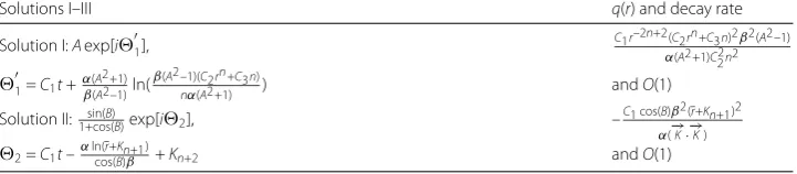
Table 1 Variable separation solution, inhomogeneity terms, and decay rate of ILLG equation (2)
Solutions I–III q(r) and decay rate
Solution I:
⎛
⎝cos(sin(11) sin() sin(BB))
cos(B)
⎞
⎠, –C1r2–2n(C2rn+C3n)2 cos(B)β2
αC22n2
1= –cos(αB)βln(–cos(B)β(αC2nrn+C3n)) +C1t andO(1)
Solution II:
⎛
⎝cos(sin(22) sin() sin(BB))
cos(B)
⎞
⎠, –C1 cos(B)β2(r+Kn+1)2
α(−→K·−→K)
2=C1t–αln(cos(r+KnB)β+1)+Kn+2 andO(1)
Table 2 Variable separation solution, inhomogeneity terms, and decay rate of equivalent ILLG equation (27)
Solutions I–III q(r) and decay rate
Solution I:Aexp[i1],
C1r–2n+2(C2rn+C3n)2β2(A2–1) α(A2+1)C2
2n2 1 =C1t+βα((AA2+1)2–1)ln(β(A
2–1)(C2rn+C3n)
nα(A2+1) ) andO(1)
Solution II: sin(B)
1+cos(B)exp[i2], –
C1 cos(B)β2(r+Kn+1)2
α(−→K·−→K) 2=C1t–αln(cos(r+KnB)β+1)+Kn+2 andO(1)
3 Solution of ILLG equation
In this section, we present some solutions of ILLG equation. These solutions are all in explicit forms, which can be seen in theorems and corollaries of this section. For
con-venience, we list all these solutions in the Tables1and2, which demonstrate the exact
solutions and their decay rates.
3.1 Solution under the cylindrical coordinates
We construct and analyze the variable separation type solution of (4) under the cylindrical coordinates. According to (4) and (11), we use the special variable separation ansatz of the solution as follows:
W=F(r)eiM(t,r), (29)
where the functionsF(r) andM(t,r) (dependent variables in parentheses) are to be deter-mined.
In the real physical model of the spin system, the inhomogeneous term of (2) and (28) are usually independent oft. Hence we just consider the caseq(t−→x) =q(r). This setting and (29) lead to the derivatives of time as follows:
–(α+βi)iWt= (α+iβ)FMteiM. (30)
The structure ofqrWris
qrWr=qreiM(iMrF+Fr). (31)
Similarly, the item associated with the Laplace and nonlinear derivatives is
q
W– 2W W¯ 2
r
1 +|W|2
=1
Adding (30)–(32) together and multiplying with e–iM, we separate their real and imagi-nary parts as we use this assumption to construct the solution of the ILLG equation, but we could not find any nontrivial solution. Hence we use another special form to find the solution of (2).
We setMin the variable separation form
M=P(r) +Q(t).
Then (33) transforms into
⎧
From the first and second equations of (34) we have
Q=C1t, (35)
whereC1is a constant.
AlthoughQis clear from (35), it is still difficult to solve (34) under the hypothesis that
Fis a function ofr. However, if we setF=A, whereAis a constant, we can simplify (34)
From the first equation of (36) we obtain
q=αC1(A 2+ 1)
P2
r(A2– 1)
By (37) the second equation of (36) transforms into
–A4Pr2βr+A4nαPr–A4Prrrα–A4αPr+ 2A2Prnα– 2A2Prrrα
– 2A2Prα+Pr2βr+Prnα–Prrrα–Prα= 0. (38)
Solving (38), we can find out the solution
P=α(A 2+ 1)
β(A2– 1)ln
β(A2– 1)(C2rn+C3n)
nα(A2+ 1)
, (39)
whereC2andC3are arbitrary constants.
Substituting (39) into (37), we obtain the exact expression ofq. According to the above analysis, we obtain the following:
Theorem 3.1 If the inhomogeneity term is
q=C1r –2n+2(C
2rn+C3n)2β2(A2– 1)
α(A2+ 1)C2 2n2
, (40)
then the solution of(28)is
W=Aexp
iα(A
2+ 1)
β(A2– 1)ln
β(A2– 1)(C2rn+C3n)
nα(A2+ 1)
+iC1t
, (41)
where A,C1,C2,and C3are constants.
Based on (40) and (41), we analyze the energy of this solution in the following contents. Ifq= 1 andn= 2, then the total energy of the solution of (28) is a constant due ton= 2
is the critical case for the LLG equation. However, if the inhomogeneity termqis not a
constant, then ILLG may not be in critical situation. We denote byE=wEdxthe total
energy of the solution of a partial differential equation.
The mapping target manifold of (28) isS2. Under projection, the conformal factor is
g= 1 (1 +|W|2)2,
whereas the energy is
∞
0
q|Wr|2grn–1dr.
Hence, the energy densitywEof (41) is
wE(41) =
αC1A2
A4– 1. (42)
Corollary 3.2 If the inhomogeneity term is
q= –C1r 2–2n(C
2rn+C3n)2cos(B)β2
αC2 2n2
, (43)
then the solution of(2)is
⎧ ⎪ ⎪ ⎨ ⎪ ⎪ ⎩
S1=cos(–C1t+cosα(B)βln(–
cos(B)β(C2rn+C3n)
αn ))sin(B),
S2= –sin(–C1t+cosα(B)βln(–
cos(B)β(C2rn+C3n)
αn ))sin(B),
S3=cos(B),
(44)
where B is a constant,and C1,C2,and C3are the same constants as in Theorem3.1.
It is clear that (44) does not tend to a trivial solution (for example, S= (0, 0, 1)) as
t→+∞. Moreover, we cannot find out a constant value oflimt→+∞S. According to Corol-lary3.2, (43) and (44) lead to
|Sr|2=S12+S22+S32
= –r
2n–2((cos(B))2– 1)α2n2C2 2 (C2rn+C3n)2(cos(B))2β2
and
wE(44) =q|Sr|2= –
C1α(sin(B))2
cos(B) . (45)
According to (42) and (45), the energy density of two systems (28) and (2) are constants that are independent of time. This fact indicates that the energy of two equivalent ILLG equations tends to +∞in the whole spacial area.
3.2 Solution under the normal coordinates
In the last subsection, we present the exact solution under the cylindrical coordinates. We study the solution under the noncylindrical cases. The solutions obtained in this section may regard as the plane wave type solution, which is different from the cylindrical case of last subsection.
First, we search the solution of (2) undern= 3. Denote byx,y,zthe different directions of space. Inspired by the last subsection, we look for the solution of (2) in the form
⎧ ⎪ ⎪ ⎨ ⎪ ⎪ ⎩
S1(t,x,y,z) =cos(M(t,x,y,z))sin(B),
S2(t,x,y,z) =sin(M(t,x,y,z))sin(B),
S3=cos(B),
(46)
From (46), (5)–(10) can be simplified to
We use the ansatz ofMas follows:
M=P(x,y,z) +Q(t) and Q(t) =C1t, (48)
whereC1is a constant.
Substituting (48) into (47), we get solution of (2) similarly. We search the solution of (2) in the form
Substituting (52) into (5)–(10), we obtain
⎧ ⎨ ⎩
α∇q· ∇P+αqP+βcos(B)q∇P· ∇P= 0, –C1–αqcos(B)∇P· ∇P+β∇q· ∇P+βqP= 0.
(53)
Solving (53),Pandqare as follows:
⎧ ⎨ ⎩
P= –αln(r+Kn+1)
cos(B)β +Kn+2,
q= –C1cos(B)β2(r+Kn+1)2 α(−→K·−→K) ,
(54)
whereKi(i= 1, 2, 3, . . .) are arbitrary constants,−→K = (K1,K2,K3, . . . ,Kn), andr=−→K · −→x.
According to (52) and (54), we obtain the solution of (2) as follows.
Theorem 3.3 If the inhomogeneity term is
q= –C1cos(B)β 2(r+K
n+1)2
α(−→K ·−→K)
, (55)
then the solution of(2)is
⎧ ⎪ ⎪ ⎨ ⎪ ⎪ ⎩
S1=cos(C1t–αlncos(r+(BK)nβ+1)+Kn+2)sin(B),
S2=sin(C1t–αlncos(r+(BK)nβ+1)+Kn+2)sin(B),
S3=cos(B).
(56)
Similarly to (44), (56) does not tend to a trivial solution as t→+∞too. Moreover,
limt→+∞Sdoes not exist. It is easy to find the solution of (27). Employing (56) and (11), we obtain the following:
Corollary 3.4 If the inhomogeneity term satisfies(55),then the solution of(27)is
W= sin(B) 1 +cos(B)exp
i
C1t–
αln(r+Kn+1) cos(B)β +Kn+2
. (57)
The energy density of the solutions presented in Theorem3.3and Corollary3.4shows
a similar property as the solutions of the previous subsection. According to Corollary3.4, we obtain
|∇S|2= (sin(B))
2α2(|−→K|) (r+Kn+1)2(cos(B))2β2
and
wE(56) =q|∇S|2= –
C1α(sin(B))2
Similarly to (45), the energy density (58) is constant. This situation will be the same for (41) and (57):
wE(57) =q |∇
W|2
(1 +|W|2)2= –
C1α(sin(B))2(cos(B) + 1)2
4cos(B) .
In this section, we present two solutions of (2) (or (27)). For convenience, we summarize some information about these solutions in Tables1and2, respectively. From these tables we can see the exact form of variable separation solution, inhomogeneity terms, and decay rates. According to the solutions of the ILLG equation in the tables, we can see thatαand
β cannot be 0 since the denominator cannot be 0. Although the solutions of the ILLG
equation does not degenerate into the trivial solutions ast→+∞, their decay rates are all independent of the spatial variable−→x. More exactly, the decay rate of the solutions for
the ILLG equation areO(1). Different from the solutions presented in our previous work
[28,29], the solutions in Tables1and2do not develop any blowup at any time.
4 Solution of Schrödinger map equation
In this section, we study the solution of the LLG equation without damping. More clearly, we setq= 1 andβ= 0 in (2). In this setting, (2) degenerates into the simple form
∂
∂tS=SS. (59)
ThereforeWsatisfies
–iWt=W–
2W
1 +|W|2 ∇W. (60)
Although (59) is simpler than (2), the solution is very rare as far as we see. For the details of the exact solution of (59), we refer the reader to [9,12,27].
4.1 Solution under the cylindrical coordinates
In the last section, we obtain some variable separation solutions such as (44) (qas (43)) and (56) (qas (55)). According to these solutions, we can see that the extreme caseα= 0 and
β= 0 are not included since the denominator is not zero. If we settle down on the variable separation form provided in the last section, what will be the solution like? Motivated by this, we consider the solution
⎧ ⎪ ⎪ ⎨ ⎪ ⎪ ⎩
S1(t,r) =cos(N(t,r))sin(G(r)),
S2(t,r) =sin(N(t,r))sin(G(r)),
S3(r) =cos(G(r)),
(61)
whereN(t,r) andG(r) are functions to be determined.
We consider the case whereq(t−→x) does not containt. Then, by (61), (2) is greatly sim-plified and transforms into
and
sin(G)cos(G)Nr2r–Grn–Grrr+sin(G)Ntr+Gr= 0, (63)
which are nonlinear partial differential equations. To solve these equations, let us assume thatNis a variable separation function,
N=M1(r) +M2(t), (64)
whereM1(r) andM2(t) depend onrandt, respectively. Substituting (64) into (62) and (63), we obtain
M2=C5t,
–sin(G)M1r+ 2cos(G)GrM1rr+sin(G)M1rn+sin(G)M1rrr= 0, (65)
and
sin(G)cos(G)M21rr–Grn–Grrr+sin(G)C5r+Gr= 0. (66)
Equations (65)–(66) are ordinary differential equations (ODEs), which are hard to solve explicitly. However, we can find out some constraints of the solution that are useful for analysis of the decay rate of the energy density. If we use
G= 2arctaneF, (67)
then (65)–(66) transform into
2M1rFre2Fr–M1re2Fn–M1rre2Fr– 2M1rrFr
+M1re2F–M1rn–M1rrr+M1r= 0 (68)
and
M12re2Fr–Fr2e2Fr+Frre2Fr+Fre2Fn–C5e2Fr–M21rr
+rFr2–Fre2F+rFrr+nFr–C5r–Fr= 0. (69)
From (68) we obtain
M1=C1+C2
r–n+1e4F+ 2e2F+ 1e–2Fdr. (70)
Substituting (70) into (69), we have
3r–2n+3e4FC22+ 2r–2n+3e2FC22+r–2n+3e6FC22– 2r–2n+3C22
– 3r–2n+3e–2FC22–r–2n+3e–4FC22–Fr2e2Fr+ e2FFrrr+Fre2Fn
We cannot find the solution of (71). However, there is some additional information aboutF. If we solve (34), then we can find
M1=
C32r–n+1
(sin(G))2dr+C4. (72)
If we setC4=C1andC2= 1/(2C3)2, then (72) and (70) will be of the same form. Substi-tuting (72) into (66), we obtain
Grr+
(n– 1)Gr
r –
cos(G)C34r–2n+2
(sin(G))3 –sin(G)C5= 0. (73)
Equation (73) is just an ODE, which is like a sine-Gordon equation. Because (73) is not a standard sine-Gordon equation, its existence details are not so clear. In fact, we rewrite (73) as
Grr=f(r,G,Gr), (74)
where
f(r,G,Gr) = –
(n– 1)Gr
r +
cos(G)C43r–2n+2
(sin(G))3 +sin(G)C5.
We consider the Cauchy problem of (74): finding a solution of equation (74) satisfying the initial conditions
G(ε) =Gε and Gr(ε) =Grε (0 <ε< +∞, 0 <Gε<π). (75)
Obviously,f(r,G,Gr) is a continuous function of all its arguments in a neighborhood of
a point (ε,Gε,Grε). Furthermore, it is not difficult to verify thatf(r,G,Gr) have bounded
partial derivatives ∂∂Gf and ∂∂Gfr in this neighborhood. Hence, a solution of (74) (or (73)) satisfying the initial conditions (75) exists and is unique. How to construct a reasonable initial condition that satisfies (74)? We just need to employ the setting (67).
Due to (72), if we obtain the solution of (73), then we can find the solution of (71). Ac-cording to the above results, we obtain the following:
Theorem 4.1 Let F be a function satisfying(71).Tthen the solution of(59)is ⎧
⎪ ⎪ ⎨ ⎪ ⎪ ⎩
S1(t,r) = 2e
F
1+e2Fcos(C1+C2
r–n+1(e2F+ 1)2e–2Fdr+C
5t),
S2(t,r) =1+e2eF2Fsin(C1+C2
r–n+1(e2F+ 1)2e–2Fdr+C
5t),
S3(r) =1–e
2F
1+e2F,
(76)
whereas
W= eFexp
i
C1+C2
r–n+1e2F+ 12e–2Fdr+C5t
(77)
Although we cannot solve (71), we can deduce some its scale asr→+∞. Substituting
Relationship (79) means thatKdetermines the limit to be a positive or negative value of
H(r) for sufficiently larger. In this situation, we have
In this case, we obtain
lim
Ifris sufficiently large, then (81) indicates that
From (61), (64), (67), and (70) we have
wE(76) =S12r+S22r+S23r
=Nr2sin(G)2+G2r
=M21rsin(G)2+G2r
= C
4 3r–2n+2 (sin(G(r)))2 +G
2
r
=4r
2–2nF2C2
2(e2F+ 4)(e2F+ e–2F)
(F2+ 1)2 +
24r2–2nF2C2 2+ 4Fr2
(F2+ 1)2 . (83)
Substituting
F=±
n
2 –
1 2
ln(Kr) (84)
into (83), we obtain
wE(76) = 16K–2r–2(–1 +n)2
ln(Kr)2r–4n+6K–2n+4C22
+ 4r–3n+5K–n+3C22+ 6r–2n+4C22K2+ 4r–n+3Kn+1C22
+r2K2nC2 2+K2
/ln(Kr)2n2– 2ln(Kr)2n
+ln(Kr)2+ 4)2. (85)
According to (85), the scale of the energy density is
wE(76)∼O(1) (n≥2)
asr→+∞.
The energy density of (77) is
wE(77) =
|Wr|2
(1 +|W|2)2 =
e2F((r–n+1)2(e4F+ 2e2F+ 1)2(e–2F)2C2 2+Fr2)
(1 + e2F)2 . (86)
Employing (84), the right side of (86) changes into
3r–2n+4+4K1K4K1C22+ 2r–2n+4+2K1K2K1C22+r–2n+4+6K1K6K1C22
– 2r–2n+4C22– 3r–2n+4–2K1K–2K1C22–r–2n+4–4K1K–4K1C22
–K12K2K1r2K1– 2K2K1r2K1K1+K1K2K1r2K1n–K2K1r2K1+2C5+K12
– 2K1+nK1–C5r2H(r). (87)
IfC5> 0 andn≥2, then the leading-order term of (87) is
and we obtain
Relation (88) shows that the scale of the energy density is
wE(77)∼
According to (90), its leading-order term is
IfC5= 0, then, asr→+∞, we have
For sufficiently larger, (92) means thatK> 0 determines the limit to be a positive or negative value ofH3(r) According to (92), we prove (89). The decay rate of energy density
From the above analysis, we can conclude that: ifFsatisfies (71), then we have
Theorem 4.2 If n≥2,then the energy densities of(76)and(77)are
4.2 Solution under the normal coordinates
Substituting (93) into (59), we obtain
Equation (95) is a nonlinear ODE. Solving the first equation of (95), we obtain
M2=C1+C2 sin(G2)
–2
dr. (96)
Employing (96), the second equation of (95) transforms into
G2rr–sin(G2)C5– transformation like (67)
G2= 2arctan
eF2,
which transforms (97) into
2eF2C22+ e–3F2C22+ 3e–F2C22– 2e3F2C22– 16eF2F22r– 16eF2F2rr
+ 16eF2C5– e7F2C22– 3e5F2C22+ 16e3F2Fr2– 16e3F2F2rr+ 16e3F2C5
+LC
For simplicity, we just consider the case ofC2
2>LC. SubstitutingF2=ln(Karctan(r)) (K> 0) into (99) and then extracting the coefficient of the highest order ofr, we obtain the coefficient ofr4(settingAr=arctan(r)),
Similarly to the proof of Theorem4.2, there exists a functionFsatisfying (99). In this setting, we obtain the following:
Theorem 4.3 Suppose there exists a function F2satisfying(99).Then the solution of (59)
is
Furthermore,if C2
2>LC,then the decay rate of energy density is
wE
(101)or(102)∼O(1)
as r→+∞.
In Tables3and4, we present the variable separation solution (and energy density) of (59) and (60), respectively. Similarly to Tables1and2, most of the decay rates of the solutions are in a scale ofO(1) in Tables3and4. The only nonconstant decay rate of the solution is the solution I in Table3. Its decay rate is related to the dimensionnas 1/rn–1. Ifn= 1, then the decay rate degenerates to the constant scaleO(1). Similarly to the solutions in Tables1
Table 3 Variable separation solution of the LLG equation without damping (see equation (59)).Fis
Table 4 Variable separation solution of the equivalent LLG equation without damping (see equation (60)).Fsatisfies (71);F2is the solution of (99)
We investigate a variable separation solution of the multidimensional ILLG equation and Schrödinger map equation. Based on the stereographic method, we deduce an equivalent ILLG equation, which can be solved exactly. Under the different ansatzs of the solutions, we obtain some explicit solutions of the modification system. The solution of this system can be changed into the solution of the ILLG equation. Hence, for the ILLG equation, we obtain two different solutions, which are all in a constant decay scale.
Ifq= 1 andβ= 0, then the ILLG equation degenerates into the Schrödinger map
equa-tion. The situation of this equation is somewhat different from the ILLG equation: the solutions obtained are in implicit forms, which are determined by nonlinear ODEs. This brings some difficulties to our analysis of the decay behavior of the solutions. Using the some heuristic method, we obtain the asymptotic scale of the functions contained in the nonlinear system. So, the decay rate of the energy density of the solutions can be charac-terized. Clearly, we obtain two different solutions of the Schrödinger map equation, which
adopt the same decay rateO(1). However, the situation of its equivalent system is
some-what different: the decay rate of radial type solution is in anrn–1(n≥2) andO(1) (n= 1) scale, whereas the plane wave type solution isO(1).
All solutions obtained in this paper are periodic in time or spatial direction. The solution of ILLG equation (or Schrödinger map equation) of type (4) just shows a periodic behavior in the time direction. Hence, if the periodic condition is imposed in the initial condition, then the ILLG equation and Schrödinger map equation contain some smooth solutions for some large initial values. In this study, the properties of the variable separation type solutions are clearer due to their straightforward and exact form. These solutions will be useful in explaining some nonlinear dynamics of stimulation in the inhomogeneous or homogeneous system that comes from the ferromagnet.
Acknowledgements
Funding
This work is supported by TianYuan Special Fund of the National Natural Science Foundation of China (No. 11426068), Project for Young Creative Talents of Ordinary University of Guangdong Province (No. 2014KQNCX228), the PhD Start-up Fund of Natural Science Foundation of Guangdong Province (No. 2014A030310330), and Fund for Science and Technology of Guangzhou (No. 201607010352). The author is also grateful to the sponsorship from China Scholarship Council.
Competing interests
The authors declare that there are no competing interests.
Authors’ contributions
All authors read and approved the final manuscript.
Publisher’s Note
Springer Nature remains neutral with regard to jurisdictional claims in published maps and institutional affiliations.
Received: 24 July 2018 Accepted: 7 September 2018 References
1. Balakrishnan, R.: On the inhomogeneous Heisenberg chain. J. Phys. C, Solid State Phys.15, 1305–1308 (1982) 2. Baleanu, D., Golmankhaneh, A.K., Golmankhaneh, A.K.: On electromagnetic field in fractional space. Nonlinear Anal.,
Real World Appl.11, 288–292 (2010)
3. Bejenaru, I., Ionescu, A., Kenig, C., Tataru, D.: Global Schrödinger maps in dimensionsd≥2: small data in the critical Sobolev spaces. Ann. Math.173, 1443–1506 (2011)
4. Chang, N.-H., Shatah, J., Uhlenbeck, K.: Schrödinger maps. Commun. Pure Appl. Math.53, 590–602 (2000)
5. Ding, Q.: Explicit blow-up solutions to the Schrödinger maps fromR2to the hyperbolic 2-spaceH2. J. Math. Phys.50,
103507 (2009)
6. Daniel, M., Porsezian, K., Lakshmanan, M.: On the integrability of the inhomogeneous spherically symmetric Heisenberg ferromagnet in arbitrary dimensions. J. Math. Phys.35, 6498–6510 (1994)
7. Ding, S.J., Wang, C.Y.: Finite time singularity of the Landau–Lifshitz–Gilbert equation. Int. Math. Res. Not. (2007). https://doi.org/10.1093/imrn/rnm012
8. Gomez-Aguilar, J.F., Baleanu, D.: Schrödinger equation involving fractional operators with non-singular kernel. J. Electromagn. Waves Appl.31, 752–761 (2018)
9. Guo, B.L., Yang, G.S.: Some exact nontrivial global solutions with values in unit sphere for two-dimensional Landau–Lifshitz equations. J. Math. Phys.42, 5223–5227 (2001)
10. Huh, H.: Blow-up solutions of modified Schrödinger maps. Commun. Partial Differ. Equ.33, 235–243 (2008) 11. He, X.M., Qian, A.X., Zou, W.M.: Existence and concentration of positive solutions for quasi-linear Schrödinger
equations with critical growth. Nonlinearity26, 3137–3168 (2013)
12. Kosevich, A., Ivanov, B., Kovalev, A.: Magnetic solitons. Phys. Rep.194, 117–238 (1990)
13. Liu, X.G.: Concentration sets of the Landau–Lifshitz system and quasi-mean curvature flows. Calc. Var. Partial Differ. Equ.27, 493–525 (2006)
14. Landau, L.D., Lifshitz, E.M.: On the theory of the dispersion of magnetic permeability in ferromagnetic bodies. Z. Sowjetunion 8 (1935). Reproduced in Collected Papers of L. D. Landau, Pergamon, New York, pp. 101–114 (1965) 15. Lin, J.Y., Lai, B.S., Wang, C.Y.: Global well-posedness of the Landau–Lifshitz–Gilbert equation for initial data in Morrey
spaces. Calc. Var. Partial Differ. Equ.54, 665–692 (2015)
16. Li, Y.X., Wang, Y.D.: Bubbling location for F-harmonic maps and inhomogeneous Landau–Lifshitz equations. Comment. Math. Helv.81, 433–448 (2006)
17. Melcher, C.: Global solvability of the Cauchy problem for the Landau–Lifshitz–Gilbert equation in higher dimensions. Indiana Univ. Math. J.61, 1175–1200 (2012)
18. Muslih, S.I., Agrawal, O.P., Baleanu, D.: A fractional Schrödinger equation and its solution. Int. J. Theor. Phys.49, 1746–1752 (2010)
19. Morales-Delgado, V.F., Gómez-Aguilar, J.F., Baleanu, D.: A new approach to exact optical soliton solutions for the nonlinear Schrödinger equation. Eur. Phys. J. Plus133, 1–18 (2018)
20. Morales-Delgado, V.F., Gómez-Aguilar, J.F., Taneco-Hernández, M.A., Baleanu, D.: Modeling the fractional non-linear Schrödinger equation via Liouville–Caputo fractional derivative. Optik162, 1–7 (2018)
21. Merle, F., Raphaël, P., Radnianski, I.: Blowup dynamics for smooth data equivariant solutions to the critical Schrödinger map problem. Invent. Math.193, 249–365 (2013)
22. Ma, X.N., Wang, P.H., Wei, W.: Constant mean curvature surfaces and mean curvature flow with non-zero Neumann boundary conditions on strictly convex domains. J. Funct. Anal.274(1), 252–277 (2018)
23. Perelman, G.: Blow up dynamics for equivariant critical Schrödinger maps. Commun. Math. Phys.330, 69–105 (2014) 24. Sun, Y., Liu, L.S., Wu, Y.H.: The existence and uniqueness of positive monotone solutions for a class of nonlinear
Schrödinger equations on infinite domains. J. Comput. Appl. Math.321, 478–486 (2017)
25. Sulem, P., Sulem, C., Bardos, C.: On the continuous limit for a system of classical spins. Commun. Math. Phys.107, 431–454 (1986)
26. Van Den Berg, J.B., Williams, J.F.: (in-)stability of singular equivariant solutions to the Landau–Lifshitz–Gilbert equation. Eur. J. Appl. Math.24, 921–948 (2013)
27. Yang, G.S., Chang, Q.S.: Limit behavior of solution for multi-dimensional Landau-Lifshitz equations with external magnetic field. Phys. Lett. A318, 270–280 (2003)
29. Zhong, P.H., Wang, S., Zeng, M.: Two blowup solutions for the inhomogeneous isotropic Landau–Lifshitz equation. J. Math. Anal. Appl.409, 74–83 (2014)
30. Zhong, P.H., Yang, G.S.: Finite time blowup of multidimensional inhomogeneous isotropic Landau–Lifshitz equation on a hyperbolic space. Comput. Math. Appl.73, 433–449 (2017)
31. Zhang, X.G., Liu, L.S., Wu, Y.H., Cui, Y.J.: Entire blow-up solutions for a quasilinearp-Laplacian Schrödinger equation with a non-square diffusion term. Appl. Math. Lett.74, 85–93 (2017)
32. Sun, F.L., Liu, L.S., Wu, Y.H.: Infinitely many sign-changing solutions for a class of biharmonic equation withp-Laplacian and Neumann boundary condition. Appl. Math. Lett.73, 128–135 (2017)
33. Wang, P.H., Wang, X.J.: The geometric properties of harmonic function on 2-dimensional Riemannian manifolds. Nonlinear Anal.103, 2–8 (2014)
34. Wang, P.H., Zhao, L.L.: Some geometrical properties of convex level sets of minimal graph on 2-dimensional Riemannian manifolds. Nonlinear Anal.130, 1–17 (2016)
35. Han, M.A., Sheng, L.J., Zhang, X.: Bifurcation theory for finitely smooth planar autonomous differential systems. J. Differ. Equ.264(5), 3596–3618 (2018)
36. Li, F.S., Gao, Q.Y.: Blow-up of solution for a nonlinear Petrovsky type equation with memory. Appl. Math. Comput.274, 383–392 (2016)
37. Meng, F.W., Shao, J.: Some new Volterra–Fredholm type dynamic integral inequalities on time scales. Appl. Math. Comput.223, 444–451 (2013)
38. Tian, H., Han, M.A.: Bifurcation of periodic orbits by perturbing high-dimensional piecewise smooth integrable systems. J. Differ. Equ.263(11), 7448–7474 (2017)
39. Li, L.Z., Meng, F.W., Zheng, Z.W.: Oscillation results related to integral average technique for linear Hamiltonian systems. Dyn. Syst. Appl.18, 725–736 (2009)
40. Li, L.Z., Meng, F.W., Zheng, Z.W.: Some new oscillation results for linear Hamiltonian systems. Appl. Math. Comput. 208, 219–224 (2009)