R E S E A R C H
Open Access
G-stability one-leg hybrid methods for
solving DAEs
P. Agarwal
1,2,3*, Iman H. Ibrahim
4and Fatma M. Yousry
4*Correspondence:
[email protected] 1Department of Mathematics,
Anand International College of Engineering, Jaipur, India
2International Center for Basic and
Applied Sciences, Jaipur, India Full list of author information is available at the end of the article
Abstract
This paper introduces the solution of differential algebraic equations using two hybrid classes and their twin one-leg with improved stability properties. Physical systems of interest in control theory are sometimes described by systems of differential algebraic equations (DAEs) and ordinary differential equations (ODEs) which are zero index DAEs. The study of the first hybrid class includes the order of convergence,
A(
α
)-stability, stability regions, and G-stability for its one-leg twin in two cases: for step (k= 1) and steps (k= 2). For the second class, G-stability of its one-leg twin is studied in two cases: for steps (k= 2) and steps (k= 3). Test problems are introduced with different step size at different end points.MSC: 65L05; 65L06; 65L20
Keywords: Hybrid methods; One-leg methods; DAEs; G-stability; A(
α
)-stability1 Introduction
Consider the initial value problems of the form
fx(t);x(t);t= 0; x(t0) –a= 0, t∈[t0;T], (1)
wherea∈Rmis a consistent initial value for (1) and the functionf:Rm×Rm×[t 0;T]→ Rm is assumed to be sufficiently smooth. If (∂f/∂x) is nonsingular, then it is possible to
formally solve (1) forxin order to obtain an ordinary differential equation. However, if (∂f/∂x) is singular, it is no longer possible and the solutionxhas to satisfy certain algebraic constraints; therefore, equations (1) are referred to as differential algebraic equations.
Systems of differential algebraic equations arise from many applications such as physics, engineering, and circuit analysis. Some systems can be reduced to an ODE system, which are zero index DAEs, and can be solved by numerical ODE methods after reduction. Other systems, in which reductions to an explicit differential systems are in the formx=f(x;t), are either impossible or impractical, that is because the problem is more naturally posed in the form
ft,x,x,y= 0; (2-a)
g(t,x,y) = 0; (2-b)
and a reduction might reduce the sparseness of Jacobian matrices. These systems are then solved directly [16,17].
A fundamentally important concept in the algorithms of the numerical solutions of DAEs is the index of a DAE. In a sense, this tells us how far away the DAE is from be-ing an ODE. The index of a DAE is the minimum number of times all or part of the DAE system must be differentiated with respect to time in order to convert the DAE into an explicit ODE. The higher the index is, the further it is from an ODE and the more difficult it is in general to solve the DAE [12].
The first general method applied to the numerical solution of DAEs is backward differ-entiation formula (BDF). Ebadi andGokhale presented in [9–11] class 2+1 hybrid BDF-like methods, hybrid BDF methods (HBDF), and new hybrid methods for the numerical solu-tion of IVPs. These methods have wide stability regions and good performance in solving CPU time compared to the extended BDF (EBDF) and modified extended BDF (MEBDF) methods [3].
In Sect.2the first hybrid class is derived, its orders of convergence are investigated, and its stability analysis is studied. In Sect.3some basic notions of one-leg schemes and G-stability are mentioned. The one-leg twin of the first class is derived and its G-G-stability is discussed in Sect.4. The one-leg twin of the second class [14] is derived and its G-stability is discussed in Sect.5. Numerical tests are investigated in Sect.6. Finally, a conclusion is introduced.
2 The first hybrid class
The first hybrid class takes the form
yn+s=hμfn+ k
j=0
γn–jyn–j, (3)
yn+ k
j=1
αn–jyn–j=h(βsfn+s+β1fn+β0fn–1), (4)
wherefn+s=f(tn+s;yn+s);tn+s=tn+sh; –1 <sandβs,β1,αn–j,j= 1, 2, . . . ,k, are parameters
to be determined as functions ofsandβ0. The methods for stepkand orderp=k+ 1 (from k= 1 up to 6) will be derived andyn+shas orderk– 1. To evaluate the value ofyn+sat an
off-step point, i.e.tn+s, we will consider the nodestn(double node),tn–1, . . . ,tn–k(simple
nodes).
Applying Newton’s interpolation formula for this data gives the following scheme:
y(t) =yn+ (t–tn)yn+ (t–tn)2
hyn–∇yn h2
+ (t–tn)2(t–tn–1)
hyn–∇yn–12∇2yn
2!h3
+ (t–tn)2(t–tn–1)(t–tn–2)
hyn–∇yn–12∇2yn–13∇3yn
Differentiate (5) with respect tot:
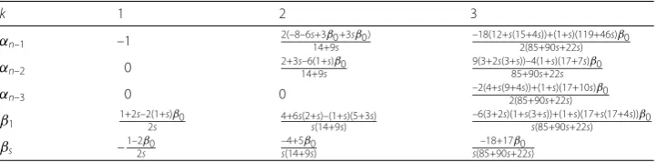
Table 1 The coefficients of method (2.2) for orders 2, 3, and 4
k 1 2 3
αn–1 –1 2(–8–6s+314+9sβ0+3sβ0) –18(12+s(15+4s))+(1+s)(119+46s)2(85+90s+22s) β0
αn–2 0 2+3s–6(1+s)14+9s β0 9(3+2s(3+s))–4(1+s)(17+7s)85+90s+22s β0
αn–3 0 0 –2(4+s(9+4s))+(1+s)(17+10s)2(85+90s+22s) β0
β1 1+2s–2(1+s)2s β0 4+6s(2+s)–(1+s)(5+3s)s(14+9s) –6(3+2s)(1+s(3+s))+(1+s)(17+s(17+4s))s(85+90s+22s) β0
βs –1–22sβ0
–4+5β0 s(14+9s)
Table 2 The coefficients of method (2.2) for order 5
k 4
αn–1 –288(48+s(78+s(36+5s)))+(1+s)(8996+6055s+985s)6(1660+s(2265+s(952+125s))) β0
αn–2 72(24+s(57+s(32+5s)))–3(1+s)(1274+s(913+155s))(3320+2s(2265+s(952+125s))) β0
αn–3 –32(8+5s)(2+s(4+s))+3(1+s)(316+s(281+55s))(3320+2s(2265+s(952+125s))) β0
αn–4
18(12+s(33+s(24+5s)))–(1+s)(374+s(367+85s))β0 6(1660+s(2265+s(952+125s)))
β1 12(24+5s(4+s)(5+s(4+s)))–3(1+s)(74+s(96+s(39+5s)))s(1660+s(2265+s(952+125s))) β0
βs s(1660+s(2265+s(952+125s)))6(–48+37β0)
Table 3 The coefficients of method (2.2) for order 6
k 5
αn–1 (–7200(120+s(231+s(142+s(35+3s))))+(1+s)(615,436+s(553,907+3s(53,483+5002s)))(12(48,076+s(77,175+s(42,980+9975s+822s)))) β0)
αn–2 (300(120+s(321+s(236+s(65+6s))))–4(1+s)(17,929+s(17,174+s(5194+501s)))(48,076+s(77,175+s(42,980+9975s+822s))) β0)
αn–3 (–400(40+s(117+s(98+3s(10+s))))+9(1+s)(2948+s(3325+s(1127+118s)))(48,076+s(77,175+s(42,980+9975s+822s))) β0)
αn–4 (225(60+s(183+s(164+s(55+6s))))–4(1+s)(5221+s(6362+3s(794+91s)))(3(48,076+s(77,175+s(42,980+9975s+822s)))) β0
αn–5 (–96(24+s(75+s(70+s(25+3s))))+(1+s)(3436+s(4379+s(1753+222s))))(4(48,076+s(77,175+s(42,980+9975s+822s)))) β0
β1 (60(5+2s)(24+s(5+s)(20+3s(5+s)))–24(1+s)(197+s(302+s(163+s(37+3s))))(s(48,076+s(77,175+s(42,980+9975s+822s)))) β0)
βs
–7200+4728β0 s(48,076+s(77,175+s(42,980+9975s+822s)))
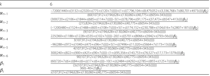
Table 4 The coefficients of method (2.2) for order 7
k 6
αn–1 –7200(1440+s(3132+s(2320+s(775+s(120+7s)))))+(1+s)(7,796,104+s(8,479,052+s(3,336,768+7s(80,701+4973s))))(60(107,912+s(194,628+s(130,060+s(40,775+s(6054+343s)))))) β0)
αn–2 (300(720+s(2106+s(1844+s(685+s(114+7s)))))–5(1+s)(78,796+s(91,175+s(37,473+s(6547+413s))))(215,824+2s(194,628+s(130,060+s(40,775+s(6054+343s))))) β0)
αn–3
(–1200(480+s(1524+s(1488+s(605+s(108+7s)))))+5(1+s)(174,152+s(230,788+s(104,616+7s(2807+187s))))β0) (9(107,912+s(194,628+s(130,060+s(40,775+s(6054+343s))))))
αn–4 225(360+s(1188+s(1228+s(535+s(102+7s)))))–20(1+s)(5701+s(8066+s(3942+s(793+56s))))3(107,912+s(194,628+s(130,060+s(40,775+s(6054+343s))))) β0
αn–5 –96(288+s(972+s(1040+s(475+s(96+7s)))))+5(1+s)(7496+s(11,020+s(5664+7s(173+13s))))4(107,912+s(194,628+s(130,060+s(40,775+s(6054+343s))))) β0
αn–6 300(240+s(822+s(900+s(425+s(90+7s)))))–(1+s)(95,356+s(143,753+s(76,527+s(17,173+1379s))))90(107,912+s(194,628+s(130,060+s(40,775+s(6054+343s))))) β0
β1 (60(720+7s(6+s)(84+s(6+s)(17+s(6+s))))–10(1+s)(2484+s(4292+s(2785+s(855+s(125+7s)))))(3s(107,912+s(194,628+s(130,060+s(40,775+s(6054+343s)))))) β0)
βs s(107,912+s(194,628+s(130,060+s(40,775+s(6054+343s)))))360(–40+23β0)
2.1 Stability analysis
Consider the scalar test problemy=λy,y(0) =y0. From equations (3) and (4) the corre-sponding characteristic equation is as follows:
yn+ k
j=1
αn–jyn–j=h
βs
hμyn+
k
j=0
γn–jyn–j
+β1yn+β0yn–1
, (9)
whereh=λy, i.e.
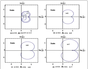
Figure 1The absolute stability domain of class (3–4) fork= 1 up to 7
where
A=βsμr, B=βs k
j=0
γn–jr1–j+β1r+β0, C=r+ k
j=1
an–jr1–j. (11)
The absolute stability regions for this class fork= 1 up to 7 are given in Fig.1for the optimalsandβ0using the boundary locus method.
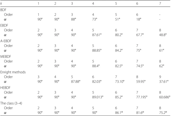
The angleαof A(α)-stability for different methods, BDF, EBDF, A-EBDF, MEBDF, En-right methods, HEBDF, and The class (3–4) for various orders are tabulated in Table5.
We recall some basic notions of one-leg schemes and G-stability.
3 One-leg schemes
Suppose that a lineark-step method
k
i=0
αiyn+i=h k
i=0
βif(tn+i,yn+i) (12)
is given. One-leg methods can be formulated in a compact form by introducing the poly-nomials
ρ(ξ) =
k
i=0
αiξi, σ(ξ) = k
i=0
Table 5 A(α)-stability for BDF, EBDF, A-EBDF, MEBDF, Enright methods, HEBDF, and The class (3–4) for various orders
k 1 2 3 4 5 6 7
BDF
Order 1 2 3 4 5 6
-α 90° 90° 88° 73° 51° 18°
-EBDF
Order 2 3 4 5 6 7 8
α 90° 90° 90° 87.61° 80.2° 67.7° 48.8°
A-EBDF
Order 2 3 4 5 6 7 8
α 90° 90° 90° 88.85° 84.2° 75° 61°
MEBDF
Order 2 3 4 5 6 7 8
α 90° 90° 90° 88.4° 82.5° 74.5° 62°
Enright methods
Order 3 4 5 6 7 8 9
α 90° 90° 87.88° 82.03° 73.10° 59.95° 37.61°
HEBDF
Order 2 3 4 5 6 7 8
α 90° 90° 90° 89.013° 85.2° 77.195° 60.686°
The class (3–4)
Order 2 3 4 5 6 7 8
α 90° 90° 90° 90° 86.1o 81.6o 75.2o
with real coefficients αi,βi∈Rand no common divisor. There is also the assumption
throughout the normalization that
σ(1) = 1. (14)
The associated one-leg methods are defined by
k
i=0
αiyn+i=hf
k
i=0
βitn+i, k
i=0
βiyn+i
. (15)
In the one-leg methods, the derivative f is evaluated at one point only, which makes it easier to analyze. The one-leg method (15) may have stronger nonlinear stability proper-ties such as G-stability [12,15]. On the other hand, it is known that to obtain a one-leg method of high order, the parametersαi,βihave to satisfy more constraints than those
for linear multistep methods, see [7,8,14]. The conditionsρ(1) = 0,ρ(1) =σ(1) = 1 imply the consistency of the scheme (ρ,σ).
3.1 G-stability analysis
The G-stability analysis, announced at the 1975 Dundee conference and published in [6], uses the test problem dy/dx=f(x,y), wherey–z,f(x,y) –f(x,z) ≤0. In the same pub-lication, one-leg methods were introduced and related to corresponding linear multistep methods. Stable behavior for this problem was defined as G-stability. A more detailed ac-count of this work will be given.
If the differential equation satisfies the one-sided Lipschitz condition
withν= 0, then the exact solutions are contractive. Consider the multistep method as a mappingRn,k→Rn,k. LetY
m= (ym+k–1, . . . ,ym)Tand consider inner product norms onRn,k
Ym 2G= k
i=1 k
j=1
gjiym+i–1,ym+j–1, (17)
where ·,·is the inner product onRn used in (16) andk-dimensional matrixG= (g ij) i,j= 1, . . . ,kis assumed to be real, symmetric, and positive definite. The inner product·,·, on which·,·Gis built, is supposed to have a corresponding norm defined by u 2=u,u.
Similarly we will write ·,· Gas the norm corresponding to·,·G.
Definition 1([6]) The one-leg method (15) is called G-stable if there exists a real, sym-metric, and positive definite matrixGsuch that, for two numerical solutions{Ym}and { ˆYm}, we have
Ym+1–Yˆm+1 G≤ Ym–Yˆm G (18)
for all step sizesh> 0 and for all differential equations satisfying (16) withν= 0.
Theorem 1([2]) G-stability implies A-stability.
Theorem 2([12]) Consider a method(ρ,σ).If there exists a real,symmetric,and positive definite matrix G,and real numbers a0, . . . ,aksuch that
1 2
ρ(ξ)σ(ω) +ρ(ω)σ(ξ)= (ξ ω– 1)
k
i,j=1
gijξi–1ωj–1+
k
i=0 aiξi
k
i=0 ajωj
, (19)
then the corresponding one-leg method is G-sable.
Theorem 3([5]) Ifρandσ have no common divisor,then the method(ρ,σ)is A-stable if and only if the corresponding one-leg method is G-stable.
4 One-leg method for the first hybrid class
Here, the one-leg twin of the first class is studied whenk= 1 andk= 2.
In the case of k= 1, method (4) takes the form
αnyn+αn–1yn–1=h(βsfn+s+β1fn+β0fn–1), (20)
yn+s=yn+shfn, (21)
where
αn= 1, αn–1= –1, βs=
–1 + 2β0
2s , and β1=
1 + 2s– 2(1 +s)β0
2s .
Method (20) has order 2, its truncation error takes the form
T2=2 + 3s– 6(1 +s)β0
12 h
The one-leg twin of (20) takes the form
αnyn+αn–1yn–1=hf(βstn+s+β1tn+β0tn–1) (22)
and has order 2 and its truncation error takes the form
T2= (1/24)h3y(3)(η).
To discuss G-stability of (22),
fn+s=fn.
Substitutefn+sin equation (20), it becomes
αnyn+αn–1yn–1=h(βsfn+β1fn+β0fn–1).
The corresponding characteristic equations are
ρ(ξ) =αnξ+αn–1, σ(ξ) = (β1+βs)ξ+β0.
Applying Theorem2, the variablesai,i= 0, 1 andgij,i,j= 1 satisfy the relations
a0=
1
2–β0, a1= –
1
2–β0 and g11=a
2 0+β0.
Chooseβ0< 1/2,g11= 1/2 > 0. So, method (22) is G-stable. In the case of k= 2, method (4) takes the form
αnyn+αn–1yn–1+αn–2yn–2=h(βsfn+s+β1fn+β0fn–1), (23)
yn+s=yn+shfn+s2(hfn–yn+yn–1). (24)
After normalization
αn=
14 + 9s
6(2 +s+ (1 +s)β0)
, αn–1=
–8 – 6s+ 3(1 +s)β0
3(2 +s+ (1 +s)β0)
,
αn–2=
2 + 3s– 6(1 +s)β0
6(2 +s+ (1 +s)β0)
βs=
–4 + 5β0
6s(2 +s+ (1 +s)β0)
, and β1=
4 + 6s(2 +s) – (1 +s)(5 + 3s)β0
6s(2 +s+ (1 +s)β0)
.
Method (23) has order 3, its truncation error takes the form
T3=
8 + 2s(9 + 4s) +β0(–21 –s(33 + 10s) + 12(1 +s)β0
72(2 +s+ (1 +s)β0)
h4y(4)(η).
The one-leg twin of (23) takes the form
and has order 2 ifβ0= (2 + 3s)/(6(1 +s)) and its truncation error takes the form
T3= (1/24)h3y(η).
To discuss G-stability of (25),
fn+s=fn+ 2s(hfn–yn+yn–1)/h.
The corresponding characteristic equations are
ρ(ξ) = (αn+ 2sβs)ξ2+ (αn–1– 2sβs)ξ+αn–2,
> 0. Therefore, the matrix G is positive definite and method (25) is G-stable.
5 The second hybrid class
The second hybrid classtakes the form
where
Method (28) has order 2, its truncation error takes the form
T3=2 + 3s(2 +s) +β
and has order 2 and its truncation error takes the form
¯
then method (30) has order 3 and its truncation error becomes
¯
The corresponding characteristic equations are
Choosingβ∗= 0.3 ands= –0.1 makesa0= –0.583636,
a1= 1.54524, a2= –0.9616, g11> 0 and
Det
g11 g12 g21 g22
> 0.
Therefore, the matrix G is positive definite and method (30) is G-stable.
In the case of k= 3, the method takes the form
αnyn+αn–1yn–1+αn–2yn–2+αn–3yn–3=hβs
fn+s–β∗fn–1
, (31)
yn+s=yn+shfn+s2(hfn–yn+yn–1), (32)
where
αn=
11 + 12s+ 3s2– 2β∗
6(1 –β∗) , αn–1=
–(6 + 10s+ 3s2+β∗)
2(1 –β∗) , αn–2=
3 + 8s+ 3s2+ 2β∗
2(1 –β∗) , αn–3=
–(2 + 6s+ 3s2+β∗)
6(1 –β∗) and βs=
1 (1 –β∗).
Method (31) has order 3 and its truncation error takes the form
T4=(3 + 2s)(1 +s(3 +s)) +β
∗
12(–1 +β∗) h
4y(4)(η).
The one-leg twin of (31) takes the form
αnyn+αn–1yn–1+αn–2yn–2+αn–3yn–3
=hfβstn+s–βsβ∗tn–1
(33)
and has order 2, its truncation error takes the form
¯
T3= – (1 +s)
2β∗
2(–1 +β∗)2h 3y(η).
To discuss G-stability of (33), using (8), we have
hfn+s=hfn+ 2s(hfn–yn+yn–1).
Substitutefn+sin equation (31), it becomes
3
i=0
αn–iyn–i=βs
hfn+ 2s(hfn–yn+yn–1)
–hβ∗fn–1
The corresponding characteristic equations are
ρ(ξ) = (αn+ 2sβs)ξ3+ (αn–1– 2sβs)ξ2+αn–2ξ+αn–3 and
σ(ξ) = (1 + 2s)βsξ3–β∗βsξ2.
Applying Theorem2, the variablesai,i= 0, 1, 2, 3 andgij;i,j= 1, 2, 3 satisfy the relations
g11=a20,
g12=g21=a0a1,
g13=g31=12a0a2(–1 +β
∗)2–β∗(2 + 3s(2 +s) +β∗)
12(–1 +β∗)2 , g23=g32
=–3(1 + 2s)(6 +s(14 + 3s)) – 12a2a3(–1 +β
∗)2+β∗(–14 – 3s(10 +s) + 2β∗)
12(–1 +β∗)2 ,
g22=a20+a21,
g33=a20+a21+2a
2
2(–1 +β∗)2–β∗(6 +s(14 + 3s) +β∗)
2(–1 +β∗)2 .
Choosings= –0.3 andβ∗= 0.2 makesa0= –0.231455;
a1= 0.613677, a2= –0.53299,
a3= 0.150767, g11> 0,
Det
g11 g12 g21 g22
> 0 and Det
⎛ ⎜ ⎝ ⎡ ⎢ ⎣
g11 g12 g13 g21 g22 g23 g31 g32 g33 ⎤ ⎥ ⎦ ⎞ ⎟ ⎠> 0.
Therefore, the matrix G is positive definite and method (33) is G-stable.
6 Numerical tests
Here, some numerical results are presented to evaluate the performance of the proposed technique [1,4,13]. The numerical tests are solved after reduction.
Test 1 Consider the differential algebraic equations:
y1(t) –ty2(t) +t2y3(t) +y1(t) – (t+ 1)y2(t) +t2+ 2ty3(t) = 0;
y2(t) –ty3(t) –y2(t) + (t– 1)y3(t) = 0; y3(t) =sin(t);
with the initial conditiony1(0) = 1;y2(0) = 1;y3(0) = 0; and the exact solution is
Test 2 Consider the differential algebraic equations:
x(t) = 2(1 –y)sin(y) +x/(1 –y); 0 =x2+ (y– 1)cos2(y);
with the initial conditionx(1) = 1;y(1) = 0; and the exact solution isx(t) =tcos(1 –t2), y(t) = 1 –t2.
Test 3 Consider the differential algebraic equations:
x(t) =f(x;t) –B(x;t)y; 0 =g(x;t);
wherex(t) = (x1,x2)T;f(x;t) = (1 + (t– 1/2)exp(t), 2t+ (t2– 1/4)exp(t))T;B(x;t) = (x 1,x2)T; g(x;t) = 1/2(x2
1+x22– (t– 1/2)2– (t2– 1/4)2); with the initial conditionx1(0) = –1/2;x2(0) =
–1/4; and the exact solution isx1(t) = (t– 1/2);x2(t) =t2– 1/4;y(t) =exp(t).
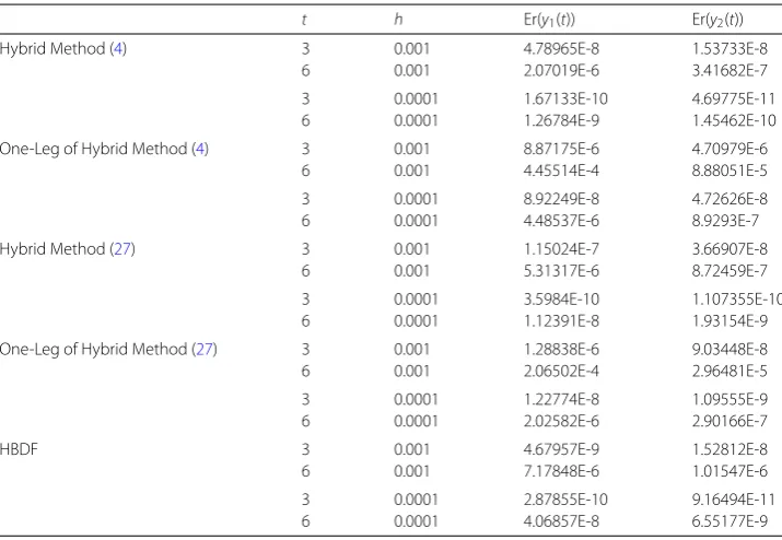
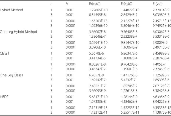
The above tests are solved by the two hybrid classes and their one-leg twins of the two classes withk= 2 at different values oft. In the first method,β0= 0.8,s= 2, and in the
second method,β∗= –0.4,s= –0.3. The errors of numerical solutions of tests1,2, and3 are tabulated in Tables6,7, and8, with different step-sizesh, respectively.
7 Conclusion
In this paper, the first hybrid class is studied fork= 1 up to 6. It has large stability regions. Its one-leg twin fork= 1 (p= 2) andk= 2 (p= 3) is G-stable. In the second class, for
k=p= 2, the one-leg twin has order 2 except whens=1 3(–3 +
√
3(1 – 2β∗+β∗2)) it has
order 3. Fork=p= 3, the one-leg twin has order 2 and ifβ∗= 0, it leads to one leg hybrid BDF, and they are G-stable. The numerical tests show that the hybrid method (4) gives good result with small steps.
Table 6 The error of the first test
t h Er(y1(t)) Er(y2(t))
Hybrid Method (4) 3 0.001 4.78965E-8 1.53733E-8
6 0.001 2.07019E-6 3.41682E-7
3 0.0001 1.67133E-10 4.69775E-11
6 0.0001 1.26784E-9 1.45462E-10
One-Leg of Hybrid Method (4) 3 0.001 8.87175E-6 4.70979E-6
6 0.001 4.45514E-4 8.88051E-5
3 0.0001 8.92249E-8 4.72626E-8
6 0.0001 4.48537E-6 8.9293E-7
Hybrid Method (27) 3 0.001 1.15024E-7 3.66907E-8
6 0.001 5.31317E-6 8.72459E-7
3 0.0001 3.5984E-10 1.107355E-10
6 0.0001 1.12391E-8 1.93154E-9
One-Leg of Hybrid Method (27) 3 0.001 1.28838E-6 9.03448E-8
6 0.001 2.06502E-4 2.96481E-5
3 0.0001 1.22774E-8 1.09555E-9
6 0.0001 2.02582E-6 2.90166E-7
HBDF 3 0.001 4.67957E-9 1.52812E-8
6 0.001 7.17848E-6 1.01547E-6
3 0.0001 2.87855E-10 9.16494E-11
Table 7 The error of the second test
t h Er(y1(t)) Er(y2(t))
Hybrid Method 1.3 0.001 6.79234E-13 4.38633E-10
2.3 0.001 3.66441E-8 1.53328E-8
1.5 0.0001 1.23906E-12 7.22089E-13
3 0.0001 7.66911E-10 1.98713E-9
One-Leg Hybrid Method 1.3 0.001 1.20205E-6 1.07885E-6
2.3 0.001 1.08490E-5 3.18015E-6
1.5 0.0001 1.54044E-8 1.13384E-8
3 0.0001 8.71812E-8 2.76648E-8
Class1 1.3 0.001 8.48159E-11 4.33369E-10
2.3 0.001 1.37322E-7 3.42503E-8
1.5 0.0001 1.41808E-12 2.87503E-12
3 0.0001 1.36406E-8 3.2887E-8
One-Leg Class1 1.3 0.001 2.17487E-7 1.48626E-7
2.3 0.001 2.25127E-6 1.99805E-6
1.5 0.0001 3.73525E-9 6.91022E-10
3 0.0001 2.8067E-7 1.95566E-6
HBDF 1.3 0.001 3.24911E-9 2.8293E-9
2.3 0.001 8.05334E-6 1.9571E-6
1.5 0.0001 4.8609E-11 3.10769E-11
3 0.0001 7.08909E-3 2.92056E-1
Table 8 The error of the third test
t h Er(x1(t)) Er(x2(t)) Er(y(t))
Hybrid Method 1 0.001 1.22665E-10 1.44872E-10 2.37014E-9
3 0.001 8.34595E-8 2.85294E-7 8.03989E-7
1 0.0001 1.63203E-13 2.12274E-13 2.45715E-12
3 0.0001 1.02396E-10 3.50464E-10 9.74921E-10
One-Leg Hybrid Method 1 0.001 3.66007E-8 9.76405E-8 6.03067E-7
3 0.001 1.38646E-7 2.52238E-7 3.53319E-6
1 0.0001 3.62941E-10 9.81447E-10 5.9809E-9
3 0.0001 3.0906E-10 1.16064E-9 2.49718E-8
Class1 1 0.001 5.5670E-6 6.86347E-6 3.45989E-5
3 0.001 3.41734E-5 1.18007E-4 2.28748E-4
1 0.0001 8.08261E-8 9.76428E-8 4.405E-7
3 0.0001 3.46347E-7 1.19601E-6 2.32459E-6
One-Leg Class1 1 0.001 6.7857E-9 1.47176E-8 1.12592E-7
3 0.001 1.69542E-7 5.4232E-7 1.85398E-6
1 0.0001 2.48221E-7 1.85705E-7 7.07125E-8
3 0.0001 3.66093E-9 1.22613E-8 3.38426E-8
HBDF 1 0.001 5.68471E-10 1.28144E-9 6.63956E-9
3 0.001 1.07333E-8 4.18462E-8 8.94225E-8
1 0.0001 7.12319E-13 1.52255E-12 6.35358E-12
3 0.0001 1.43312E-11 5.25517E-11 1.13875E-10
Acknowledgements
We are really thankful to the reviewers for their useful suggestions and corrections.
Funding
Not applicable.
Abbreviations
Availability of data and materials
Not applicable.
Competing interests
The authors declare that they have no competing interests.
Authors’ contributions
All authors contributions are equal and they all read and approved the final manuscript.
Author details
1Department of Mathematics, Anand International College of Engineering, Jaipur, India.2International Center for Basic
and Applied Sciences, Jaipur, India.3Department of Mathematics, Harish-Chandra Research Institute (HRI), Allahbad, India.4Department of Mathematics, Faculty of Women for Arts, Science and Education, Ain Shams University, Cairo, Egypt.
Publisher’s Note
Springer Nature remains neutral with regard to jurisdictional claims in published maps and institutional affiliations.
Received: 20 September 2018 Accepted: 12 February 2019
References
1. Ascher, U., Lin, P.: Sequential regularization methods for nonlinear higher index DAEs. SIAM J. Sci. Comput.18, 160–181 (1995)
2. Baiocchi, C., Crouzeix, M.: On the equivalence of A-stability and G-stability. Appl. Numer. Math.5, 19–22 (1989) 3. Cash, J.R.: Modified extended backward differentiation formulae for the numerical solution of stiff initial value
problems in ODEs and DAEs. J. Comput. Appl. Math.125, 117–130 (2000)
4. Celik, E.: On the numerical solution of differential-algebraic equation with index-2. Appl. Math. Comput.156, 541–550 (2004)
5. Dahlquist, G.: G-stability is equivalent to A-stability. BIT Numer. Math.18, 384–401 (1978)
6. Dahlqusit, G.: Error analysis for a class of methods for stiff nonlinear initial value problems. In: Numerical Analysis Dundee. Lecture Notes in Mathematics, vol. 506, pp. 60–74. Springer, Berlin (1975)
7. Dahlqusit, G.: Some properties of linear multistep and one-leg methods for ODEs. In: Skeel, R.D. (ed.) Proc. 1979 SIGNUM Meeting on Numerical ODEs (1979) Report R 79/963
8. Dahlqusit, G., Liniger, W., Nevanlinna, O.: Stability of two step methods for variable integration steps. SIAM J. Numer. Anal.20, 1071–1085 (1983)
9. Ebadi, M., Gokhale, M.Y.: Hybrid BDF methods for the numerical solutions of ordinary differential equations. Numer. Algorithms55, 1–17 (2010)
10. Ebadi, M., Gokhale, M.Y.: Class 2 + 1 hybrid BDF-like methods for the numerical solutions of ordinary differential equations. Calcolo48, 273–291 (2011)
11. Ebadi, M., Gokhale, M.Y.: A class of multistep methods based on a super-future points technique for solving IVPs. Comput. Math. Appl.61, 3288–3297 (2011)
12. Hairer, E., Lubich, C., Roche, M.: The Numerical Solution of Differential-Algebraic Systems by Runge–Kutta Methods. Lecture Notes in Mathematics, vol. 1409. Springer, Berlin (1989)
13. Husein, M.M.J.: Numerical solution of linear differential-algebraic equations using Chebyshev polynomials. Int. Math. Forum3(39), 1933–1943 (2008)
14. Ibrahim, I.H., Yousry, F.M.: Hybrid special class for solving differential algebraic equations. Numer. Algorithms69(2), 301–320 (2015)
15. Liniger, W.: Multistep and one-leg methods for implicit mixed differential algebraic system. IEEE Trans. Circuits Syst.
26(9), 755–762 (1979)
16. Michael, H., Roswitha, M., Caren, T., Ewa, W., Stefan, W.: Least-squares collocation for linear higher-index differential–algebraic equations. J. Comput. Appl. Math.317, 403–431 (2017)