R E S E A R C H
Open Access
available at the end of the articleAbstract
This paper deals with the dynamic behavior of the chaotic nonlinear time delay systems of general formx˙(t) =g(x(t),x(t–
τ
)). We carry out stability analysis to identify the parameter zone for which the system shows a stable equilibrium response. Through the bifurcation analysis, we establish that the system shows a stable limit cycle through supercritical Hopf bifurcation beyond certain values of delay and parameters. Next, a numerical simulation of the prototype system is used to show that the system has different behaviors: stability, periodicity and chaos with the variation of delay and other parameters, which demonstrates the validity of our method. We give the single- and two-parameter bifurcation diagrams which are employed to explore the dynamics of the system over the whole parameter space.Keywords: Bifurcation analysis; Periodicity; Chaos; Hopf bifurcation
1 Introduction
For the last decades, time-delayed dynamical systems have been attracting the attention of researchers of various fields, including mathematics, biology, economics, physics, engi-neering, etc. [1–4]. Many natural systems are mathematically modeled by nonlinear delay differential equations which contain one or more time delays. Successful examples include blood production in patients with leukemia [5], dynamics of optical systems [6,7], popula-tion dynamics [8], physiological model [9], El Niño/southern oscillation [10], the Lorentz force with Liénard–Weichert potentials [11], neural network with three neurons [12], de-lay feedback control and synchronization [13,14], etc. The presence of a delay in a system makes the system infinite-dimensional, and may lead to an unstable and oscillatory re-sponse. In particular, the time delay of a nonlinear system may give rise to various complex phenomena such as bifurcation, chaos, hyperchaos, multistability, etc.
There are many reasons why the nonlinear delay dynamical systems have been stud-ied in the mathematical modeling of the naturally occurring phenomena [15,16]. Firstly, the delay differential equations show higher-dimensional chaotic behavior which cannot be anticipated by a low-dimensional system [17]. It is important to understand and ex-plore the behavior of these systems both from the academic and engineering perspective. Secondly, infinite dimensionality of delayed systems offers a great opportunity to the re-searchers to harness the richness of hyperchaos, having multiple positive Lyapunov expo-nents. It has been proved that communication with a low-dimensional chaos is not fully secure because an eavesdropper can reconstruct chaotic attractors and retrieve a hidden
message [18,19]. Therefore, the synchronization of hyperchaotic systems has been pro-posed as an alternative method for improving the security in the communication schemes [20–22]. It has been proved that a simple time delay system with suitable nonlinearity can produce a hyperchaotic signal with multiple positive Lyapunov exponents, thus making it a good candidate for a secure communication system [23,24]. Beside a secure communica-tion system, chaotic and hyperchaotic systems have important applicacommunica-tions in chaos-based noise generators [25], improvement of motion capabilities and of sensors in robotics [26,
27], etc.
Hence, the bifurcation analysis of time-delay chaotic systems has been the subject of worldwide attention in the last decades [28]. In [29], Campbella and Ncubeb gave an ex-plicit description of the region of stability for a linear scalar delay differential equation consisting of two arbitrarily distributed time delays. El-Dessoky et al. investigated the lo-cal Hopf bifurcation in Shimizu–Morioka chaotic system with delayed feedback control [30]. Song et al. studied the stability and Hopf bifurcation in a model of gene expression with distributed time delays [31]. In [32], Feng and Wei investigated the effect of delayed feedbacks on the generalized Sprott B system with hidden attractors and its local Hopf bifurcation. Atay and Ruan studied systems of coupled units in a general network con-figuration with a coupling delay [33]. Yeniceri and Yalcin introduced the first generaliza-tion for time-delay sampled-data chaotic system in order to generate multiscroll attractors [34]. Wei et al. made a lot of contributions to the Hopf bifurcation analysis of many equa-tions, such as Mackey–Glass system [35], delayed Nicholson blowflies equation [36], and a neural network model with delay [37]. We would like to mention that there are several papers on the bifurcation formed by a branch of periodic orbits of a family functional dif-ferential equations, see Dormaer [38,39], and the global existence of periodic solutions in delayed differential equations based on the global Hopf bifurcation theory given by Wu [40]; for example, see the works given by Ruan and Wei [41], Song and Wei [42], Wen and Wang [43]. Tang et al. casted light on network synchronous state stability via studying the bifurcation (or transition) problem of network synchronized regions with varying nodal dynamics [44]. Xiao et al. proposed a delayed fractional-order congestion control model which is more accurate than the original integer-order model when depicting the dual congestion control algorithms [45].
In this paper, we first study a general chaotic nonlinear time delay system with a constant time delay. We carry out stability analysis to identify the parameter zone for which the system shows a stable equilibrium response. Through the bifurcation analysis, the system shows a stable limit cycle through supercritical Hopf bifurcation beyond certain values of delay and parameters of the system. Next, a numerical simulation of the prototype system shows that the system shows stability, periodicity and chaos with the variation of delay and other system parameters. We give the single- and two-parameter bifurcation diagrams which are employed to explore the dynamics of the system over the whole parameter space. The numerical results demonstrate the validity of our method.
2 Stability and bifurcation analysis
2.1 The system description
For a discussion of the stability analysis, we consider the following delay differential equa-tion:
˙
x(t) =gx(t),x(t–τ) (t≥t0) (1)
whereτ ≥0 is the time delay, andg is a function ofx(t) andx(t–τ). Equation (1) is of very general nature because of the functiong, which can be linear, piecewise linear, or nonlinear. A few particular cases of this system are Mackey–Glass equationx˙(t) = –bx+
axτ/(1 +xcτ) arising in the model of leukemia [46], Ikeda equationx˙(t) =bx(t) +asin(cxτ)
in optics [47], and the piecewise linear Lu–He modelx˙(t) = –ax(t) +bf(xτ) [48], where
f(x) is a piecewise linear function. Heret0is the initial interval andτ > 0 corresponds to
the delay time, which represents the time interval between the start of an event at one point and its resulting action at another point in the system. The solution of the system equation defined in (1) is determined uniquely when an initial functionφ(t) defined on an initial interval is prescribed as
x(t) =φ(t), fort∈[t0–τ,t0]. (2)
The time delay is approximated or its effects are generally ignored by modelers. Several researches have commented on the dangers modelers risk if they ignore delays which they think are small [49]. In the case of approximation used for the delay elements, their effects on the system behavior can only be partly observed. The delay elements arise naturally in various diverse fields: chemical kinetics, infectious diseases, and the navigational control of ships and aircraft [49]. Therefore, the subject of differential equations with time delay is now a rapidly growing field, and numerical solution of systems modeled by delay differ-ential equations is both of theoretical and practical interest. The bibliography prepared by Baker et al. shows recent developments and interests in this field [50].
In this paper, we first discuss the stability and bifurcation analysis of the above nonlinear continuous delay system (1). Through the bifurcation analysis, we establish that the system shows a stable limit cycle through supercritical Hopf bifurcation beyond certain values of delay and system parameters. Next, a numerical simulation of the considered nonlinear system [51,52] is used to show that the system exhibits stability, periodicity and chaos with the variation of delay and other system parameters, which demonstrates the validity of the proposed theory. The nonlinear continuous system in dimensionless form with one-state variable is as follows:
˙
x(t) =γx(t–τ) –βfx(t–τ), (t≥t0), (3)
2.2 Stability analysis of delay differential equation
Consider the delay differential equation (1), namelyx˙(t) =g(x(t),x(t–τ)). The equilibrium pointsx∗are obtained by solving
gx∗,x∗= 0. (4)
Then, we consider the linearization of the system near the equilibriumx∗. Defining a small perturbationξ=x–x∗to equilibrium solution and using Taylor’s approximation, we get a linearized equation of (1) as
˙
As we known, an equilibrium pointx∗is asymptotically stable if all rootsλiof the
char-acteristic equation (6) satisfy
Re(λi) < 0, ∀i. (7)
If the delay timeτ= 0, the eigenvalue isλ=a+b. Condition (7) then takes the forma+b< 0, which implies that the equilibrium pointx∗ is stable. In the following we consider the delay timeτ= 0. Hopf bifurcation will appear if at least one of the eigenvalues crosses the imaginary axis from the left and enters the right half-plane. Puttingλ=μ+iω, ifμvaries from the left to right, we can say thatμ< 0 is a stable state,μ> 0 is a bifurcated state, and
μ= 0 is the limiting case. At the emergence of Hopf bifurcation, we putμ= 0. Thus using
λ=iω, we have
iω=a+be–iωτ. (8)
Now equating the real and imaginary parts on both sides of the above equation, we obtain
thenλk(τ) =μk(τ) +iωk(τ) is a root of (6) satisfyingμτk= 0 andωk(τk) =ω0. We have the
following results.
Lemma 1 μk(τk) > 0.
Proof Differentiating both sides of (6) with respect toτ, it follows that
dλ
Hence,ddμτ > 0 on each of the critical surfacesτk, which implies that there does not exist
any eigenvalue with a negative real part across the critical surface. Thus, there is only one possible stability region (under the conditiona+b< 0) enclosed byτ= 0 and the critical surfaceτ0.
Then, we have the following main conclusion:
Case I. Ifa+b< 0 thenτ= 0 gives stable solutions. Further, the stability surfaces exist if
b2>a2. (16)
The stability region is bounded by the planeτ= 0 and the closest critical surfaceτ0.
If condition (16) is not satisfied, then the stability properties will not change in this re-giona+b< 0, i.e., the solutions are stable for anyτ≥0.
Case II. Ifa+b> 0 then the system will be unstable for anyτ≥0 and for any parameter
values.
We summarize these conclusions in the following theorem.
Theorem 1 Suppose x∗is an equilibrium solution of the delay differential equation(1),
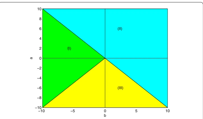
Figure 1Stability regions of Eq. (1): (I) stable region for the delay in the interval [0,τ1(0)), (II) unstable region,
(III) stable region
Proof Claim 1. It is followed fromb∈(–∞, –|a|) thata+b< 0 andb2>a2. The equation
has a pair imaginary roots±iω0whenτ =τk(k= 0, 1, 2, . . . ). Ifτ∈[0,τ0), all the roots of
equation (1) have negative real parts, i.e., the equilibriumx∗is stable. The statement on the number of eigenvalues with positive real parts follows from Lemma1and Rouché’s theorem [53].
Claim 2. It follows fromb∈(–a, +∞) thata+b> 0, and then the equation has at least one root with a positive real part for allτ≥0, i.e., for equation (1), the equilibrium point
x∗is unstable for allτ≥0.
Claim 3. It follows fromb∈(a, –a) thata+b< 0 andb2<a2. For allτ≥0, all the roots
of the equation have negative real parts, i.e., the equilibriumx∗is stable. These results are also summarized in Fig.1.
3 Stability analysis of the prototype model
The system given in (3) has been used as a prototype model to observe self-oscillations in the shipbuilding industry [54]. In [51], the author studies the basic chaotic behavior by numerical simulation. For theoretically analyzing the complexity of the system given by (1), we rewrite (3) in the following form [52]:
˙
x(t) =gx(t),xτ
=γx(t–τ) –βx3(t–τ), (17) whereγ andβ are positive parameters of the system andτ is the time delay. The equi-librium condition implies x˙= 0 and x(t) =x(t–τ) =x∗, i.e.,g(x∗,x∗) =γx∗–βx∗3= 0.
This implies that the system has three equilibrium points, namely the originE1= 0 and
E2,3=±
√
γ/β. Based on the analysis of [40,55,56], we will find the value ofτ where the fixed point losses its stability through Hopf bifurcation. From (17), one has
J0=
∂g(x(t),xτ)
and
Jτ=
∂g(x(t),xτ) ∂xτ
=γ– 3βx2(t–τ). (19)
In the following, our aim is to examine the stability of every equilibrium point.
3.1 Stability of the equilibrium pointE1
In this section, we consider the stability of the equilibrium pointE1= 0. Since we have
J0|E1= 0 andJτ|E1=γ, the characteristic equation is given by
J0+Jτe–λτ–λ=γe–λτ–λ= 0, (20)
which implies
λ=γe–λτ. (21)
If the delay timeτ= 0, the eigenvalueλ=γ > 0, which implies that the equilibrium point
E1= 0 is unstable. Ifτ= 0, the conclusion can be obtained by Theorem1as follows:
Theorem 2 Equation(21)has at least one root with a positive real part for allτ≥0,i.e.,
for equation(17),the equilibrium point E1= 0is unstable for allτ≥0.
Proof Sincea=J0|E1= 0 andb=J1|E1 =γ > 0, we havea+b=γ > 0, which implies that
equation (21) has at least one root with a positive real part for allτ > 0. Hence, the equi-librium pointE1= 0 is unstable forτ ≥0.
3.2 Stability of the equilibrium pointsE2,3
In this section, we study the stability of the equilibrium pointsE2,3=±
√
γ/βby the same method. Since we haveJ0|E2,3= 0 andJτ|E2,3=γ – 3β
γ
β = –2γ, the characteristic equation
is given by
J0+Jτe–λτ–λ= –2γe–λτ–λ= 0, (22)
which implies
λ= –2γe–λτ. (23)
If the delay time τ = 0, the eigenvalueλ= –2γ < 0, which implies that the equilibrium pointsE2,3=±√γ/βare stable. In the following, we consider the delay timeτ = 0. Hopf
bifurcation will appear if at least one of the eigenvalues crosses the imaginary axis from the left and enters the right half-plane. Puttingλ=μ+iω, ifμvaries from the left to right, we can say thatμ< 0 is a stable state,μ> 0 is a bifurcated state, andμ= 0 is the limiting case. At the emergence of Hopf bifurcation, we putμ= 0, thus usingλ=iω, we have
Now equating the real and imaginary parts on both sides of above equation, we obtain
Proof Differentiating both sides of (23) with respect toτ, it follows that
dλ
Lemma 3 For the equilibrium points E2,3,there exists a sequence of values ofτ
0 <τ0<τ1<· · ·<τk<· · ·, (32)
such that(i)equation(23)has a pair imaginary roots±iω0whenτ=τk (k= 0, 1, 2, . . . ),
(ii)ifτ∈[0,τ0),all the roots of equation(23)have negative real parts,ifτ=τ0,all roots of
equation(23)except±iω0have negative real parts,and ifτ∈(τk,τk+1)for k= 0, 1, 2, . . . ,
Proof From (25) and (26), we obtain that equation (23) has purely imaginary roots±iω0if
and only ifτ =τk. The statement about the number of eigenvalues with positive real parts
in (ii) follows from Lemma2and Rouché’s theorem [53].
Theorem 3 The equilibrium points E2,3= 0are asymptotically stable forτ ∈[0,τ0)and
unstable forτ>τ0,and equation(17)undergoes a Hopf bifurcation at E2,3whenτ=τkfor
= 0, 1, 2, . . . .
Proof This theorem can be proof by Lemma3. It also can be obtained by Theorem1with
b∈(–∞, –|a|), wherea= 0 andb= –2γ < 0. In this section, we have the conclusion: (i) equation (17) is unstable forτ ≥0 at the equilibrium pointE1; (ii) equation (17) is asymptotically stable forτ∈[0,τ0) and unstable
forτ>τ0at the equilibrium pointsE2,3, and equation (17) undergoes a Hopf bifurcation
at the equilibrium pointsE2,3whenτ=τkfor = 0, 1, 2, . . .
4 Numerical simulation
In the previous section, we obtained that the considered equation atE2,3is asymptotically
stable forτ ∈[0,τ0) and unstable forτ >τ0, and equation (17) undergoes a Hopf
bifur-cation at E2,3when τ =τk fork= 0, 1, 2, . . . . In the following, we will give the dynamic
behaviors of the system with different parameterγ and different time delayτ. And the bifurcation diagrams will be obtained by plotting the local maxima ofx, excluding a large number of transients. System (17) is solved numerically using the fifth-order Runge–Kutta algorithm with integration step sizeh= 0.005 and the constant initial functionφ(t) = 0.1 fort∈[–τ, 0].
4.1 The dynamic behavior with
γ
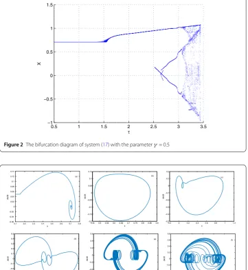
= 0.5First, we vary the time delayτ, takingγ = 0.5 andβ= 1. Whenτ ≥1.57, the fixed point loses its stability through Hopf bifurcation, which is in accordance with the analysis of the previous section. The bifurcation diagram is shown in Fig.2. According to the numerical simulations and Fig.2, we find that the system is asymptotically stable forτ∈[0, 1.57). The limit cycle of period-1 becomes unstable and a period-2 cycle appears atτ= 2.54. Further period doubling occurs at τ = 2.65 (period-2 to period-4). Through a period doubling sequence, the system enters into the chaotic region atτ= 3.1. At last, the system becomes divergent atτ= 3.45. A phase plane representation in the representativex–dx/dtplane for differentτ is shown in Fig.3, which shows the following characteristics: stability (τ= 1), period-1 (τ= 1.8), period-2 (τ = 2.6), period-4 (τ= 2.7), and chaos (τ= 3.1 andτ= 3.3).
4.2 The dynamic behavior with
γ
= 1Now we study the dynamic behavior of system (2) by varying the time delayτand taking
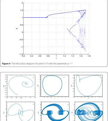
γ = 1 andβ= 1. Whenτ≥0.79, the fixed point loses its stability through Hopf bifurcation, and the bifurcation diagram is shown in Fig.4. According to the numerical simulations and Fig.4, the following conclusions are found. The system is asymptotically stable for
Figure 2The bifurcation diagram of system (17) with the parameterγ= 0.5
Figure 3The phase plane plot inx–dx/dtspace for differentτ: (a)τ= 1 (stability), (b)τ= 1.8 (period-1), (c)τ= 2.6 (period-2), (d)τ= 2.7 (period-4), (e)τ= 3.1 (chaos), (f)τ= 3.3 (chaos) with parameterγ= 0.5
system becomes divergent atτ = 1.72. A phase plane representation in the representative
x–dx/dtplane for differentτis shown in Fig.5, which shows the following characteristics: stability (τ = 0.5), period-1 (τ = 0.9), period-2 (τ = 1.3), period-4 (τ = 1.35), and chaos (τ= 1.55 andτ = 1.65).
4.3 The dynamic behavior with
γ
= 1.5Figure 4The bifurcation diagram of system (17) with the parameterγ= 1
Figure 5The phase plane plot inx–dx/dtspace for differentτ: (a)τ= 0.5 (stability), (b)τ= 0.9 (period-1), (c)τ= 1.3 (period-2), (d)τ= 1.35 (period-4), (e)τ= 1.55 (chaos), (f)τ= 1.65 (chaos) with parameterγ= 1
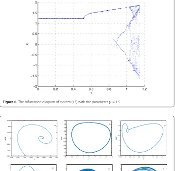
the system enters into the chaotic regime atτ = 1.01. Then, the system enters into the divergent region atτ= 1.15. A phase plane representation in the representativex–dx/dt
plane for differentτ is shown in Fig.7, which shows the following characteristics: stability (τ = 0.3), period-1 (τ = 0.6), period-2 (τ= 0.87), period-4 (τ = 0.9), and chaos (τ = 1.03 andτ= 1.1).
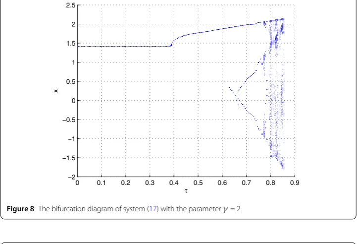
4.4 The dynamic behavior with
γ
= 2Then we study the dynamic behaviors of system (2) by varying the time delayτand taking
Figure 6The bifurcation diagram of system (17) with the parameterγ= 1.5
Figure 7The phase plane plot inx–dx/dtspace for differentτ: (a)τ= 0.3 (stability), (b)τ= 0.6 (period-1), (c)τ= 0.87 (period-2), (d)τ= 0.9 (period-4), (e)τ= 1.03 (chaos), (f)τ= 1.1 (chaos) with parameterγ= 1.5
cycle appears atτ= 0.64. Further period doubling occurs atτ = 0.66 (2 to period-4). Through a period doubling sequence, the system enters into the chaotic region atτ= 0.76. At last, the system becomes divergent atτ = 0.86. A phase plane representation in the representativex–dx/dtplane for differentτ is shown in Fig.9, which shows the following characteristics: stability (τ= 0.25), period-1 (τ = 0.45), period-2 (τ= 0.65), period-4 (τ= 0.68), and chaos (τ= 0.77 andτ= 0.83).
4.5 The dynamic behavior with
γ
= 2.5In the following, we study the dynamic behaviors of system (2) when we vary the time delay
Figure 8The bifurcation diagram of system (17) with the parameterγ= 2
Figure 9The phase plane plot inx–dx/dtspace for differentτ: (a)τ= 0.25 (stability), (b)τ= 0.45 (period-1), (c)τ= 0.65 (period-2), (d)τ= 0.68 (period-4), (e)τ= 0.77 (chaos), (f)τ= 0.83 (chaos) with parameterγ= 2
is asymptotically stable forτ ∈[0, 0.31). And the limit cycle of period-1 becomes unsta-ble and a period-2 cycle appears atτ = 0.51. Further period doubling occurs atτ = 0.53 (period-2 to period-4). Through a period doubling sequence, the system enters into the chaotic region atτ= 0.61. Then, the system becomes divergent atτ= 0.69. A phase plane representation in the representative x–dx/dtplane for differentτ is shown in Fig.11, which shows the following characteristics: stability (τ = 0.2), period-1 (τ = 0.36), period-2 (τ= 0.52), period-4 (τ = 0.54), and chaos (τ= 0.62 andτ= 0.66).
4.6 The dynamic behavior with
γ
= 3In the end, we study the dynamic behavior of system (2) when we vary the time delayτ
Figure 10 The bifurcation diagram of system (17) with the parameterγ= 2.5
Figure 11 The phase plane plot inx–dx/dtspace for differentτ: (a)τ= 0.2 (stability), (b)τ= 0.36 (period-1), (c)τ= 0.52 (period-2), (d)τ= 0.54 (period-4), (e)τ= 0.62 (chaos), (f)τ= 0.66 (chaos) with parameterγ= 2.5
Figure 12 The bifurcation diagram of system (17) with the parameterγ= 3
Figure 13 The phase plane plot inx–dx/dtspace for differentτ: (a)τ= 0.17 (stability), (b)τ= 0.3 (period-1), (c)τ= 0.43 (period-2), (d)τ= 0.46 (period-4), (e)τ= 0.52 (chaos), (f)τ= 0.55 (chaos) with parameterγ= 3
4.7 The dynamical behavior of the system over the whole
τ
–γ
parameter spaceUsing the bifurcation analysis theory and the results of numerical simulation, the following conclusions are found: (i) the system is asymptotically stable forτ ∈[0,π/(4γ)); (ii) the system has periodic solutions whenτ ∈(π/(4γ), 6.08/(4γ)); (iii) the system has chaotic behaviors whenτ∈(6.08/(4γ), 6.88/(4γ)); (iv) the system is divergent whenτ> 6.88/(4γ). The results are given in Fig.14. The regions (I)–(IV) indicate the stable, periodic, chaotic, and divergent zones of the system, respectively.
5 Conclusions
Figure 14 The different regions in theτ–γparameter space with parameterβ= 1
numerical simulations of the prototype system to demonstrate the validity of our method. The numerical simulations with the variation of time delay prove that the system shows a period-doubling route to chaos. And we study the dynamical behaviors of the system over the wholeτ–γ parameter space. Then, we give four different regions (I)–(IV) where the system shows stable, periodic, chaotic, and divergent behavior, respectively. In the future work, we will study the limit cycles and homoclinic/heteroclinic orbits in our system.
Funding
This work is supported by Natural Science Foundation of China (Grant No. 11701397, 61573010), Sichuan Youth Science & Technology Foundation (No. 2016JQ0046), Artificial Intelligence Key Laboratory of Sichuan Province (No. 2016RYJ06), Fund of Sichuan University of Science and Engineering (No. 2016RCL33, 2015RC10), Opening Project of Key Laboratory of Higher Education of Sichuan Province for Enterprise Informationalization and Internet of Things (No. 2016WYJ04).
Competing interests
The authors declare that they have no competing interests.
Authors’ contributions
The main idea of this paper was proposed by TL. YW and XZ prepared the manuscript initially and performed all the steps of the proofs in this reserch. All authors read and approved the final manuscript.
Author details
1School of Mathematics and Statistics, Sichuan University of Science and Engineering, Zigong, China.2Artificial
Intelligence Key Laboratory of Sichuan Province, Zigong, China.3Key Laboratory of Higher Education of Sichuan Province
for Enterprise Informationalization and Internet of Things, Zigong, China.4Yellow River Conservancy Technical Institute,
Kaifeng, China.
Publisher’s Note
Springer Nature remains neutral with regard to jurisdictional claims in published maps and institutional affiliations.
Received: 29 July 2018 Accepted: 1 November 2018
References
1. Wang, Z.: A numerical method for delayed fractional-order differential equations. J. Appl. Math.2013, 2560711–2560717 (2013)
2. Wang, Z., Huang, X., Zhou, J.P.: A numerical method for delayed fractional-order differential equations: based on G-L definition. Appl. Math. Inf. Sci.7(2), 525–529 (2013)
4. Li, Y., Zhang, W.H., Liu, X.K.: Stability of nonlinear stochastic discrete-time systems. J. Appl. Math.2013, 3567461–3567468 (2013)
5. Mackey, M.C., Glass, L.: Oscillation and chaos in physiological control system. Science197, 287–289 (1977)
6. Ikeda, K., Daido, H., Akimoto, O.: Optical turbulence: chaotic behavior of transmitted light from a ring cavity. Phys. Rev. Lett.45, 709–712 (1980)
7. Wei, J., Yu, C.: Stability and bifurcation analysis in the cross-coupled laser model with delay. Nonlinear Dyn.66, 29–38 (2011)
8. Pei, Y., Li, S., Li, C.: Effect of delay on a predator–prey model with parasitic infection. Nonlinear Dyn.63, 311–321 (2011) 9. Pei, L., Wang, Q., Shi, H.: Bifurcation dynamics of the modified physiological model of artificial pancreas with insulin
secretion delay. Nonlinear Dyn.63, 417–427 (2011)
10. Boutle, I., Taylor, R.H.S., Romer, R.A.: El Niño and the delayed action oscillator. Am. J. Phys.75, 15–24 (2007) 11. Driver, R.D.: A neutral system with state dependent delay. J. Differ. Equ.54, 73–86 (1984)
12. Liao, X., Guo, S., Li, C.: Stability and bifurcation analysis in tri-neuron model with time delay. Nonlinear Dyn.49, 319–345 (2007)
13. Le, L.B., Konishi, K., Hara, N.: Design and experimental verification of multiple delay feedback control for time delay nonlinear oscillators. Nonlinear Dyn.67, 1407–1418 (2012)
14. Kwon, O.M., Park, J.H., Lee, S.M.: Secure communication based on chaotic synchronization via interval time varying delay feedback control. Nonlinear Dyn.63, 239–252 (2011)
15. Li, G., Ling, W.Z., Ding, C.M.: A new comparison principle for impulsive functional differential equations. Discrete Dyn. Nat. Soc.10, 1–6 (2015)
16. Li, Y.X., Huang, X., Song, Y.W., Lin, J.N.: A new fourth-order memristive chaotic system and its generation. Int. J. Bifurc. Chaos25(11), 1550151 (2015)
17. Banerjee, T.: Single amplifier biquad based inductor-free Chua’s circuit. Nonlinear Dyn.68, 565–573 (2012) 18. Perez, G., Cerdeira, H.: Extracting messages masked by chaos. Phys. Rev. Lett.74, 1970–1973 (1995) 19. Li, T.Z., Wang, Y., Luo, M.K.: Control of fractional chaotic and hyperchaotic systems based on a fractional order
controller. Chin. Phys. B23, 0805011–08050113 (2014)
20. Peng, J.H., Ding, E.J., Ding, M., Yang, W.: Synchronizing hyperchaos with a scalar transmitted signal. Phys. Rev. Lett.76, 904–907 (1996)
21. Li, T.Z., Wang, Y., Yang, Y.: Synchronization of fractional-order hyperchaotic systems via fractional-order controllers. Discrete Dyn. Nat. Soc.2014, 4089721–40897214 (2014)
22. Li, T.Z., Wang, Y., Yang, Y.: Designing synchronization schemes for fractional-order chaotic system via a single state fractional-order controller. Optik125, 6700–6705 (2014)
23. Kye, W.H., Choi, M., Kurdoglyan, M.S., Kim, C.M., Park, Y.J.: Synchronization of chaotic oscillators due to common delay time modulation. Phys. Rev. E70, 0462111 (2004)
24. Wang, Y., Li, T.Z.: Synchronization of fractional order complex dynamical networks. Physica A428, 1–12 (2015) 25. Ando, B., Graziani, S.: Stochastic Resonance: Theory and Applications. Kluwer, Norwell (2000)
26. Fortuna, L., Frasca, M., Rizzo, A.: Chaotic pulse position modulation to improve the efficiency of sonar sensors. IEEE Trans. Instrum. Meas.52, 1809–1814 (2003)
27. Buscarino, A., Fortuna, A., Frasca, M., Muscato, G.: Chaos does help motion control. Int. J. Bifurc. Chaos17, 3577–3581 (2007)
28. Wang, Z., Huang, X., Shi, G.D.: Analysis of nonlinear dynamics and chaos in a fractional order financial system with time delay. Comput. Math. Appl.62(3), 1531–1539 (2011)
29. Campbella, S., Ncubeb, I.: Stability in a scalar differential equation with multiple, distributed time delays. J. Math. Anal. Appl.450, 1104–1122 (2017)
30. El-Dessoky, M., Yassen, M., Aly, E.: Bifurcation analysis and chaos control in Shimizu–Morioka chaotic system with delayed feedback. Appl. Math. Comput.243, 283–297 (2014)
31. Song, Y., Han, Y., Zhang, T.: Stability and Hopf bifurcation in a model of gene expression with distributed time delays. Appl. Math. Comput.243, 398–412 (2014)
32. Feng, Y., Wei, Z.: Delayed feedback control and bifurcation analysis of the generalized Sprott B system with hidden attractors. Eur. Phys. J. Spec. Top.224, 1619–1636 (2015)
33. Atay, F., Ruan, H.: Symmetry analysis of coupled scalar systems under time delay. Nonlinearity28, 795–824 (2015) 34. Yeniceri, R., Yalcin, M.: Multi-scroll chaotic attractors from a generalized time-delay sampled-data system. Int. J. Circuit
Theory Appl.44, 1263–1276 (2016)
35. Wei, J., Fan, D.: Hopf bifurcation analysis in a Mackey–Glass system. Int. J. Bifurc. Chaos17, 2149–2157 (2007) 36. Wei, J., Li, M.: Hopf bifurcation analysis in a delayed Nicholson blowflies equation. Nonlinear Anal., Theory Methods
Appl.60, 1351–1367 (2005)
37. Wei, J., Yuan, Y.: Synchronized Hopf bifurcation analysis in a neural network model with delays. J. Math. Anal. Appl.
312, 205–229 (2005)
38. Dormaer, P.: Smooth symmetry breaking bifurcation for functional differential equations. Differ. Integral Equ.5, 831–854 (1992)
39. Dormaer, P.: Smooth bifurcation of symmetric periodic solutions of functional differential equations. J. Differ. Equ.82, 109–155 (1989)
40. Wu, J.: Symmetric functional differential equations and neural networks with memory. Trans. Am. Math. Soc.350, 4799–4838 (1998)
41. Ruan, S., Wei, J.: Periodic solutions of planar systems with two delays. Proc. R. Soc. Edinb.129A, 1017–1032 (1999) 42. Song, Y., Wei, J.: Local Hopf bifurcation and global existence of periodic solutions in a delayed predator–prey system.
J. Math. Anal. Appl.301, 1–21 (2005)
43. Wen, X., Wang, Z.: The existence of periodic solutions for some model with delay. Nonlinear Anal., Real World Appl.3, 567–581 (2002)
44. Tang, L.K., Lu, J.A., Lu, J.H., Wu, X.Q.: Bifurcation analysis of synchronized regions in complex dynamical networks with coupling delay. Int. J. Bifurc. Chaos24(1), 14500111–145001113 (2014)
46. Mackey, M.C., Glass, L.: From Clocks to Chaos: The Rhythms of Life. Princeton University Press, Princeton (1988) 47. Ikeda, K., Matsumoto, K.: High-dimensional chaotic behavior in systems with time-delayed feedback. Physica D29,
223–235 (1987)
48. Lu, H., He, Z.: Chaotic behavior in first-order autonomous continuous-time systems with delay. IEEE Trans. Circuits Syst.43, 700–702 (1996)
49. Baker, T.H., Paul, C.A.H., Wille, D.R.: Issues in the numerical solution of evolutionary delay differential equations. Adv. Comput. Math.3, 171–196 (1995)
50. Baker, T.H., Paul, C.A.H., Wille, D.R.: A bibliography on the numerical solution of delay differential equation. Numerical Analysis Report No. 269, Mathematics Department, University of Manchester, UK (1995)
51. Ucar, A.: On the chaotic behaviour of a prototype delayed dynamical system. Chaos Solitons Fractals16, 187–194 (2003)