Novel learning based spatial reuse optimization in dense WLAN deployments

R E S E A R C H A R T I C L E

Open Access

Novel learning-based spatial reuse

optimization in dense WLAN deployments

Imad Jamil

, Laurent Cariou

and Jean-François Hélard

Abstract

To satisfy the increasing demand for wireless systems capacity, the industry is dramatically increasing the density of the deployed networks. Like other wireless technologies, Wi-Fi is following this trend, particularly because of its increasing popularity. In parallel, Wi-Fi is being deployed for new use cases that are atypically far from the context of its first introduction as an Ethernet network replacement. In fact, the conventional operation of Wi-Fi networks is not likely to be ready for these super dense environments and new challenging scenarios. For that reason, the high efficiency wireless local area network (HEW) study group (SG) was formed in May 2013 within the IEEE 802.11 working group (WG). The intents are to improve the “real world” Wi-Fi performance especially in dense deployments.

In this context, this work proposes a new centralized solution to jointly adapt the transmission power and the physical carrier sensing based on artificial neural networks. The major intent of the proposed solution is to resolve the fairness issues while enhancing the spatial reuse in dense Wi-Fi environments. This work is the first to use artificial neural networks to improve spatial reuse in dense WLAN environments. For the evaluation of this proposal, the new designed algorithm is implemented in OPNET modeler. Relevant scenarios are simulated to assess the efficiency of the proposal in terms of addressing starvation issues caused by hidden and exposed node problems. The extensive simulations show that our learning-based solution is able to resolve the hidden and exposed node problems and improve the performance of high-density Wi-Fi deployments in terms of achieved throughput and fairness among contending nodes.

Keywords: IEEE 802.11, WLAN, High density, High efficiency WLAN (HEW), MAC, Spatial reuse, Artificial neural networks

1 Introduction

Today, IEEE 802.11 wireless local area network (WLAN) [1] that is widely known as Wi-Fi is the dominant stan-dard in WLAN technology. An infrastructure mode of a basic IEEE 802.11 network is termed a basic service set (BSS) and consists of an access point (AP) and at least one associated station (STA). According to the IEEE 802.11 standard, the multiple access to the communi-cation medium is based on the contention between the different nodes operating on the same frequency channel. The distributed coordination function (DCF) manages

*Correspondence: [email protected]

The principal part of this work was done when Laurent Cariou was at Orange Labs, France

1Orange, 4 Rue de Clos Courtel, 35510 Cesson-Sevigne, France

3Institute of Electronics and Telecommunications of Rennes (IETR)—Institut National des Sciences Appliquées (INSA) de Rennes, 20 Avenue des Buttes de Coesmes, 35708 Rennes, France

Full list of author information is available at the end of the article

the contention-based access by implementing the carrier sense multiple access with collision avoidance (CSMA-CA) mechanism. As described in the standard, if a node is transmitting, all the nodes located in its transmission range must defer their transmissions. This behavior is ruled by the physical carrier sensing (PCS) that is a part of the clear channel assessment (CCA) mechanism. Accord-ingly, at a given time, there is only one communication occurring within the same BSS. Usually, this communi-cation occurs between the AP and one of the associated STAs and may take one of the two directions: downlink (DL) towards the STA or uplink (UL) towards the AP.

If the contending nodes belong to different BSSs, we talk about an overlapping BSS (OBSS) problem where the nodes of the neighboring co-channel BSSs overhear each other. When multiple co-channel BSS overlap, the com-munication airtime is shared between them and hence the total capacity of the network is divided by the number of these OBSSs. Since the number of orthogonal frequency

channels available for the operation of Wi-Fi networks is limited to 3 in the 2.4-GHz band and may reach a maximum of 24 channels in the 5-GHz band, prevent-ing OBSSs is very challengprevent-ing especially in dense WLAN environments. The impact of the increasing density on the adaptive channel selection schemes is studied in [2]. Adding to this quantitative limitation, the fact that an interference-free operation on these unlicensed channels is not always guaranteed because many other systems are using them.

Since its introduction in 1997, the IEEE WLAN stan-dard is continuously evolving. Increasing the peak phys-ical throughput was always the main intent behind this evolution. However, the achievable network throughput in real world is affected by many factors that are mostly related to the MAC layer protocols. On another hand, the focus of the standardization activity was mainly on enhancing the performance in a single BSS. Neverthe-less, in reality, the inevitable presence of OBSSs aggravates the spectral efficiency and hence the performance of the system.

The increasing demand on high-throughput, large capacity, and ubiquitous coverage for high data rate, real-time, and always-on applications is driving the wireless industry. To respond to these demands, the density of the deployed Wi-Fi networks is drastically increasing in all the deployment scenarios: indoor or outdoor public hotspots, business offices, and private residences. For instance, by 2018, the number of hotspots will grow to the equivalent average of one Wi-Fi hotspot for every 20 people on earth according to a recent study [3].

Along with this unprecedented level of density, more new challenging deployment scenarios are expected to appear. Already, Wi-Fi is seen as the most suitable solution to cover large venues, stadiums, airports, train stations, and other crowded spaces in indoor and outdoor. Further-more, Wi-Fi access points are being deployed in plains, trains, and ships. Satisfying this variety of use cases is not a simple task especially when a certain level of quality of experience (QoE) is expected to be met. To deal with the presented issues, the high efficiency WLAN (HEW) study group (SG) [4] was launched and led to the cre-ation of a new task group (TG) in May 2014 that took the name of IEEE 802.11ax [5]. The main goal of this TG is improving the spectrum efficiency to enhance the system area throughput in high-density scenarios in terms of the number of APs and/or STAs.

As argued by many researchers and standardization contributers [6–8], the current MAC protocols are very conservative when operating in dense environments. Because of this overprotecting behavior, the performance of the current high-density WLAN networks is degraded. As previously discussed, this density will continue to increase and the future networks will be more and more

vulnerable to performance degradation. Obviously, opti-mizing these protocols for more spatial reuse will boost the overall performance of high-density WLANs in terms of achieved throughput. This is why enhancing the spa-tial reuse is one of the hot topics discussed in the IEEE 802.11ax task group. Accordingly, the IEEE 802.11ax spa-tial reuse (SR) ad hoc group is created to work on improv-ing spatial frequency reuse and other mechanisms that enhance the concurrent use of the wireless medium by multiple devices. Several interesting propositions are pre-sented in this group. However, conserving the fairness among different nodes is not always assured with the cur-rently proposed solutions [9, 10]. In a previous work [11], we proposed an adaptive distributed scheme to enhance the network performance in densely deployed WLANs by leveraging the spatial reuse.

In the same context, in the aim of leveraging the spatial reuse in dense WLAN environments, this work envi-sions the adaptation of the MAC protocols of a managed WLAN system in a centralized manner. Since the next Wi-Fi generation is intended to be carrier oriented, the future Wi-Fi infrastructure will be increasingly deployed in a planned manner like cellular networks. The centralized approach, subject of this work, is appropriate for plenty of current and future Wi-Fi deployment scenarios. One of the most relevant scenarios studied in the current IEEE 802.11ax task group is the stadium scenario. Actually, two scenarios out of a total of four scenarios discussed in this task group are fully managed (see [12]).

In this paper, we exploit a new artificial neural network (ANN)-based solution to apply jointly a physical carrier sensing adaptation (PCSA) and a transmit power control (TPC) in a way that preserves fairness between all the nodes in terms of throughput. ANNs [13] are commonly used to address a wide range of pattern recognition prob-lems [14] including classification, clustering, and regres-sion. However, the worth of ANNs to model complex and nonlinear problems is desirable for many real-world prob-lems. In telecommunications domain, ANNs are adopted for a large number of applications [15], such as equalizers, adaptive beam-forming, self-organizing networks, net-work design and management, routing protocols, local-ization, etc. Furthermore, many data mining techniques make use of ANNs to derive meaning from complicated or imprecise data. In WLAN, the main applications of ANNs can be classified as follows: data rate adaptation [16], qual-ity of service (QoS) provisioning [17], frame size adapta-tion [18], channel allocaadapta-tion [19], channel estimaadapta-tion [20], and indoor localization [21].

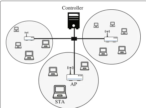
Controller

AP

STA

Fig. 1Managed wireless LAN topology former by several basic service sets (BSS) controlled by a centralized entity (the controller)

from all the nodes attached to the system (normally via their corresponding APs) in a periodic manner. The IEEE 802.11k amendment [22] that describes the mechanisms for APs and STAs to dynamically measure and report their radio resources can be useful to design the feedback col-lection function. In this work, the feedback data consists of the values of the adapted parameters and the average throughput achieved by every node. After the collection phase, the collected data is used by the ANN to learn the nonlinear relation between the parameters in input and the corresponding throughputs in output. The trained ANN is then used to adapt the parameters in such a way to minimize a predefined cost function.

The envisioned approaches to improve the spatial reuse in dense WLANs are presented in Section 1.1. In

Section 1.2, we introduce the ANNs theory and the role they play in the proposed solution. Then, the system model is detailed in Section 1.3. The proposed optimiza-tion technique is presented in Secoptimiza-tion 1.4 before explain-ing the implementation of the whole system in details in Section 1.5. For the evaluation part, Section 1.6 describes the simulation scenarios and discusses the obtained results. Finally, the paper is concluded in Section 2.

1.1 Spatial reuse in dense WLANs

In order to enhance the performance of WLANs in dense deployment scenarios, improving spatial reuse is com-pulsory. In cellular deployments, the most important approaches are prudent site planning and emerged chan-nel assignment for each cell. Although these solutions are always efficient for traditional networks, they are no more sufficient for current dense WLAN environments. Sat-isfying the tremendously increasing demand in capacity is not possible without densifying network deployments, i.e., installing more APs to serve more STAs. However, as explained earlier, due to the contention-based access mechanism, the number of concurrent transmissions is largely reduced when co-channel APs are closer to each other (OBSS problem). In these circumstances, multiple approaches are envisioned to enhance the situation. In the following, we describe the TPC and the PCSA in the light of their advantages and drawbacks. Then, we present a previous work [11] that proposes a combination of them.

1.1.1 Transmit power control (TPC)

Decreasing the transmission power of the possible inter-ferers helps to fulfill the required SINR at the neighboring receivers. As shown in Fig. 2, theoretically, the same SINR can be obtained by decreasing the transmission power of all the devices of “x dB” which leads to decrease also

the interference power by “x dB”. In that way, the trans-mission ranges in the neighboring networks are shrunk. Widely used in mobile networks, TPC is one of the pow-erful mechanisms to shrink cells while densifying and hence to permit more spatial reuse. By the same logic, TPC is suggested for high-density WLANs. While TPC is very effective when applied in fully managed architectures over licensed spectrum, many drawbacks are shown when applying it to less managed networks. WLAN deploy-ments are known to be chaotic since in most cases, the APs are individually installed. As the frequency spec-trum is unlicensed, managed networks cannot guarantee interference-free operation. In practice, any AP (even if it is a soft AP, i.e., tethering applications) operating in vicin-ity may disturb the performance of the managed network at any time.

The selflessness of TPC prevents WLAN administrators and producers from activating it when there is no punctual regulatory need (e.g., operating on a frequency band that interferes with neighboring radar systems). Authors in [23, 24] and [25] show the detrimental effect of asymmet-rical links caused by the application of TPC in some case scenarios. Actually, TPC is more problematic to achieve in a distributed manner or when the spectrum is free because it fosters higher power transmitters, that are not applying it, at the expense of lower power transmitters that are applying TPC.

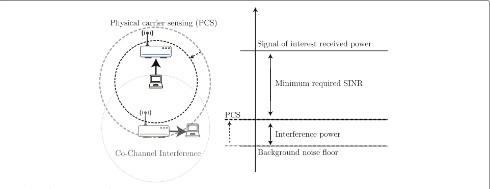
1.1.2 Physical carrier sensing adaptation (PCSA)

For the reasons discussed above, another approach that is more suitable to the contention-based access of WLAN is proposed. This approach is called PCSA and is based on the adaptation of the carrier sensing mechanism used by the CCA procedure. In PCSA, instead of decreasing its transmission power, a node will decrease its sensitiv-ity in detecting signals in its environment. In Fig. 3, the

PCS threshold is increased so that tolerable concurrent transmissions are prohibited from triggering busy channel assessments. Consequently, in situations where the sig-nal of interest is received with a power sufficiently higher than the interference power, the reuse between neighbor-ing networks will be possible. In contrast to TPC, there is an important incentive for network administrators and equipment vendors to apply PCSA since the benefit goes directly to the devices that applies it.

1.1.3 Balanced TPC and PCS adaptation (BTPA)

However, as shown in [11], there are some fairness issues when adopting one of the previous approaches alone. More precisely, it has been shown that while TPC favors the legacy devices (that are not applying TPC), PCSA favors the devices that applies the adaptation. In real world networks, the devices implementing the latest ver-sion of the 802.11 standard operate in the same networks with older devices (legacies). The interoperability and backward compatibility is an essential feature in 802.11 WLAN. Preserving fairness between different devices (particularly with legacies) is important for the overall network performance.

Consequently, we proposed in [11] the balanced TPC and PCS adaptation (BTPA). The proposal defines a mechanism to calculate two adaptation valuesTPCand PCS based on the power level received from the cor-responding peer device (i.e., the AP in UL). According to the proposal, the transmission power is reduced by TPCwhile the PCS threshold is increased byPCS. This leads to an optimal protection range around the trans-mitter X where one node transmits at a given instance. Outside this range, co-channel nodes are able to success-fully transmit simultaneously withX. In a dense cellular deployment simulation scenario, the proposed technique is able to ameliorate the fairness in different situations,

while improving the average throughput by four times compared to the standard performance.

Although BTPA could be applied in both distributed and centralized network architecture, in fully managed deployments, we can take benefit from the presence of a central controller to conceive more intelligent solutions. In the present work, we design and implement a central-ized learning-based solution that uses also an approach based on a joint adaptation of transmission power and car-rier sensing. This new solution benefits from the ANN’s ability to model complex nonlinear functions to intelli-gently enhance the spatial reuse while preserving fairness.

1.2 Introduction to artificial neural networks

Artificial neural networks (ANNs) [13] derive their com-puting power through their parallel distributed structure that gives them the ability to learn and therefore to gen-eralize by producing reasonable outputs for new unseen inputs. The properties of ANN are summarized as the fol-lowing: input-output mapping capability, adaptivity, non-linearity, and fault tolerance.

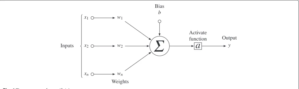
1.2.1 An artificial neuron

The artificial neuron is the basic block of an ANN. The architecture of this fundamental processing unit is shown in Fig. 4. Accordingly, the transfer function through a single neuron is defined as follows:

y=a

whereyis the output of the neurone,a(.)is the activation function,nis the number of inputs to the neuron, wi is the weight of inputi,xiis the value of inputi, andbis the bias value. Depending on the problem that the ANN needs to solve, the activation function can be a step function, a linear function, or a nonlinear sigmoid function.

1.2.2 An artificial neural network

An ANN is obtained by combining multiple artificial neu-rons. These single neurons are distributed over several layers, namely input, hidden, and output layers. The num-ber of hidden layers and the interconnections between dif-ferent neurons can be defined in difdif-ferent ways resulting in different ANN topologies [13]. Building the topology of an ANN is just half of the task before being able to use this ANN to solve the given problem. An ANN needs to learn how to respond to given inputs. The learning (or train-ing) step can be achieved in a supervised, unsupervised, or reinforcement way. The unsupervised approach consists on setting the weights and biases to values that minimize a predefined error function.

1.2.3 The weights update

In the training phase, the training data is fed into inputs, then the output of a neuron is calculated as described in Eq. (1). This procedure is repeated for all neurons at the input layer, then at the hidden layer(s), and finally at the output layer. Afterwards, the error values are calculated based on the desired output value and the actual output value. This error is used to update the weights of all the connections in the ANN. This update is done by a back propagation of the error value, meaning that the weights connecting the output layer neurons to the last hidden layer neurons are updated in the first place. When all the weights are updated, the ANN is ready for the next epoch of the training phase. The maximum number of epochs is predefined depending on the specific problem and the available dataset. The commonly used error function is the mean squares error (MSE) that is defined by

MSE= 1

(desired_outputm_i −current_outputm_i ))

(2)

whereMis the number of training datasets. When the cal-culated value of the MSE is less or equal to the predefined

desired MSE (MSEdes), the training is stopped and the ANN is considered as sufficiently trained. Furthermore, the stop point may be controlled by other customized metrics.

1.2.4 Why artificial neural networks?

The impact of the MAC protocols on the network perfor-mance is very complicated to model. Usually, researchers provide a set of unrealistic assumptions of ideal chan-nel conditions and homogeneous link qualities to simplify their studies. However, these assumptions result in biased results that do not reflect the real life situations. Conse-quently, optimization efforts basing on these impractical models result in inefficient solutions.

The relation between the individually achieved through-puts for every node and the MAC parameters used on every node is nonlinear, complex, and time variant which is very difficult to predict using an analytical model [26]. This is the motivation behind the use of ANNs to model this highly complicated relation. When the network is sufficiently trained, it will model the aforementioned rela-tion between outputs and inputs. This model can be used to minimize a cost function to determine the best MAC parameter values for each node in order to enhance the performance of the network. For this optimization, we have to define a real-time learning and adaptation algorithm.

1.2.5 Related applications of artificial neural networks in the literature

In the literature, artificial neural networks are employed to model nonlinear relationship between the inputs and the outputs of a given system. The power of neural net-works resides in their capability to approximate nonlinear functions. In [27], authors consider a multi-layered feed-forward neural network as a “universal approximator”.

Typical problems addressed by neural networks include pattern recognition, clustering, data compression, signal processing, image processing, and control problems. In telecommunications, ANNs are implemented for many applications, such as equalizers, adaptive beam-forming, self-organizing networks, network design and manage-ment, routing protocols, and localization. ANNs are also proposed in the literature to enhance the perfor-mance of WLANs. In [16], authors propose an adap-tation of the transmission data rate based on ANN to improve the aggregate throughput of a WLAN sys-tem. QoS provisioning is addressed in [17] using fuzzy logic control to enhance the IEEE 802.11e enhanced distributed channel access (EDCA) function [28] and frame size adaptation [18]. Other important applications of the ANN theory in WLAN systems include indoor localization [21], channel estimation [20], and channel allocation [19].

An adaptive algorithm is proposed in [29] to satisfy a predefined user throughput requirement by optimizing some back-off mechanism parameters. Precisely, the min-imum contention window (CWmin) and the arbitration inter-frame spacing (AIFS) are chosen as the adaptable parameters. After propagating the current values of these parameters over a multilayer neural network, the corre-sponding output is compared to the desired throughput to calculate the training error. Once the MSE is satis-fied, the trained neural network is used to optimize the input parameters using a back-propagation mechanism. This optimization consists in minimizing the following cost-reward function:

where Ti is the result of the forward-propagation over the ANN andT_Thri is the required user throughput of useri.

1.3 The proposed system model

In this work, we chose the multilayer perception (MLP), the most common ANN topology [13]. We consider an ANN topology of three layers: the input layer, one hid-den layer, and the output layer. As shown in Fig. 5, the input layer contains 2kneurons, wherek is the number of WLAN nodes in the network. Since we are consider-ing the joint optimization of the PCS threshold (PCSthr) and the transmit power (Txp), then we need to adapt 2k parameters (two parameters for each WLAN node). The output layer consists ofkneurons because we consider the throughput achieved by every node.

By the means of this ANN, we aim to model the correla-tion funccorrela-tioncf(.)between the throughput (Thr) achieved by the different WLAN nodes of the network and their associated MAC parameters.

(Thr1, Thr2,. . ., Thrk)=cf(PCSth1,Tx_p1, PCSth2,Txp2,

. . ., PCSthk,Txpk)

(4)

The aim of this study is to enhance the performance of the network in terms of throughput and preserving fairness between nodes. To chose the new adapted param-eters, a minimization of the following cost function is proposed.

Fig. 5Proposed neural network topology

of a set of throughput values whereK is the number of nodes andxi is the throughput achieved at theith node. The values generated by the Jain’s index have a range between 0 and 1, where a value of 1 means the best fair-ness. Minimizing the Cost function in Eq. (5) is the same as approaching 1 for the Jain’s index.

Although the aim is to preserve fairness in individual achieved throughput, we have to maintain a minimum average throughput per device. Accordingly,XTis defined as the individual average throughput target. BelowXT, the average throughput achieved by a given device needs to be enhanced. To satisfy this throughput requirement, we need to minimize the expression described in Eq. (6).

CostT = K

i=1

(XT−xi)2

XT

(6)

For the final cost (Eq. 7) used by the proposed algo-rithm, the previously defined costs are summed together. The term multiplied by CostT is used to normalize it so that it will produce the same weight in the total cost as Costfairness.

Costtot=Costfairness+ 1 K

i=1

XT

CostT (7)

1.4 The new optimization algorithm—updating the MAC parameters

For the(n+1)th adaptation, theith MAC parameter is adapted by incrementing or decrementing it byβ_i(n).

β(n+1)

i =β(

n)

i +β( n)

i (8)

where 1 ≤ i ≤ 2K at layer l = 0. To minimize the cost function with respect toβ_i(n), according to the gradi-ent descgradi-ent optimization technique,β_i(n)is equal to the negative gradient of the cost function as follows:

β(n)

i = −η δCost

δβ(n)

i

(9)

where ηis the update rate of the optimization process. Introducing the activation function at layer (l) to Eq. (9), we obtain

δCost δβ(n)

i

= − δCost

δa(_in)(l)×

δa(_in)(l)

δβ(n) i

(10)

Let us consider

λ(n) i (l)= −

δCost

δa(_in)(l) (11)

Fig. 7General procedure

Table 1ANN creation

Symbol Metric Description

Input Metrics to optimize PCS threshold and transmission power of each node

Output Achieved throughput Average throughput of each node

At the output layer (l=2),λ(_in)(l)is given by

λ(n) i (2)= −

δCost

δa(_in)(2) (12)

where theδa(_in)(2)is the activation function value calcu-lated at the output layer after the feed forward process

previously described.λ(_in)(0)are then derived fromλ(_in)(1) that are derived from λ(_in)(2), all using the chain-rule manner described by

λ(n)

i (l)= Nl+1

j=1 λ(n)

j (l+1)aj(l+1)wij(l+1) (13)

accordingly, we have

λ(n) i (0)= −

δCost δa(_in)(0) = −

δCost δβ(n)

i

(14)

sincea(_in)(0)(the ith input of the ANN) is equal toβ_i(n) (the current value of the ith parameter). Equation (8) becomes

β(n+1)

i =β

(n) i +ηλ

(n)

i (0) (15)

Our proposal reposes on the expression of Eq. (15) to calculate the new adapted parameters during the opti-mization process.

1.5 Implementation of the proposed solution

We used OPNET modeler 17.5 as the simulation tool. OPNET is a system level simulator that implements the PHY and MAC layers described by the IEEE 802.11n stan-dard. The essential procedures of the proposed solution are described in this section.

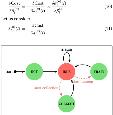
A new OPNET node model is created to simulate the controller entity. The process model is represented by its finite state machine shown in Fig. 6. The ANN is created in the initialization phase INIT, then the process enters the IDLE state and remains there until the next scheduled collection time. The collection event releases the process that enters the COLLECT state. At the end of the collec-tion procedure, the process returns to the IDLE state and waits for the training event. Once fired, process goes to the TRAIN state, trains the ANN, and returns to the IDLE state.

1.5.1 Overview on the proposed solution

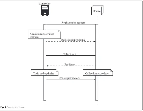
As shown in Fig. 7, each device has to send a registra-tion request to the controller. Upon receipt of this request, the controller creates a registration context specific to the requesting device. The controller affirms or denies the registration with an appropriate registration response. A newly associated device can have the latest optimized parameters via this response.

At a predefined moment, the controller sends a col-lection start command to all the registered devices. The collection procedure is described in details in the next section. After collecting all the datasets, the controller performs an online training for the previously created neural network. Then, the trained neural network is used to adapt the parameters of the devices. The optimization procedure is described later in this paper.

Finally, the controller sends the optimized parameters values to the corresponding devices. After receiving the update parameters request, each device applies the new parameters and continues its normal operation. Accord-ing to the circumstances and the predefined policies, the controller is able to send a new collection command whenever it needs.

1.5.2 The different procedures of the proposed algorithm

After examining every procedure apart from others, the overall algorithm is shown in Fig. 8. The optimization

round consists of returning to the start step after run-ning through the different steps depicted in the flowchart. An optimization roundnbegins by an initialization phase where the ANN is created and configured (Table 1). Then, the current version of the training dataset is fetched. As it will be described in detail later on, initially, the offline dataset is divided randomly into two parts, one is a part of the training dataset and the other constitutes the test-ing dataset. The fetched dataset is the offline traintest-ing part appended to the previously collected dataset entries

during past optimization rounds (< n). Then, a new col-lection procedure starts and the resulting dataset entry is appended to the fetched training dataset. At this point, we are ready to proceed to the training phase described in Section 1.5.3. After that, the ANN is tested using the testing dataset as outlined in Section 1.5.4. If the resulting testing MSE increases’ compared to that of the previous optimization round (n −1), the process quits the training phase and enters the optimization procedure (see Section 1.5.5). At the end of the optimization pro-cedure, the process returns to the start point and a new optimization round (n+1) starts.

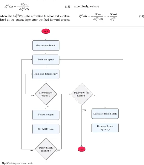
1.5.3 Training procedure

In this section, we describe the training procedure of the ANN. The latter is based on two types of datasets, the first is collected offline (when the real network is not in oper-ational mode) and the second is the result of an online collection (while the normal system operation).

The offline datasetis divided into two separate datasets. The first part is used as the initial part of the training dataset, while the second part is used to test the ANN during the training process. The testing procedure is an important player in determining the end of the training process and the beginning of the optimization process.

The online dataset is the complementary part of the training data set. After every optimization round, the collected dataset entry is appended to the latest train-ing dataset. Accordtrain-ingly, the ANN is trained with an

incremental training dataset, increasing in size after each optimization round. This assures an adaptive behavior of the proposed solution.

The detailed training procedure is depicted in Fig. 9. To increase the robustness of the training phase, we inte-grate two test levels to verify if the network is successfully trained or not. To implement our approach, we consider two different criteria. One of them is the well-known desired mean square error (MSEdes). The other criteria is the number of output errors exceeding certain abso-lute value (the desired fail limit FLdes) that is equivalent to the difference between the output neuron value and the related value in the dataset. We define the desired fail number ratio FNrdes as the ratio of output errors exceed-ing FLdes to the total number of output values in the training dataset (number of ANN’s outputsK times the number of dataset entries DSenb). Accordingly, the first test level consists of a verification whether the current MSE value is less than MSEdes value. Once the desired MSE is satisfied, we move to the second test level by test-ing the number of fails. If the latter does not satisfy the predefined FNdes value, the MSEdesand the learning rate μare decreased.

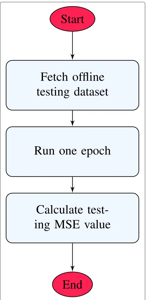
1.5.4 Testing procedure

The testing procedure consists of fetching the offline test-ing dataset entries and runntest-ing the ANN for one epoch. Obviously, this run will not affect the trained ANN, mean-ing that the weights are not updated. Consequently, the

testing MSE value is calculated to be used later to con-clude if the ANN is enough trained or not. Figure 10 depicts the described procedure.

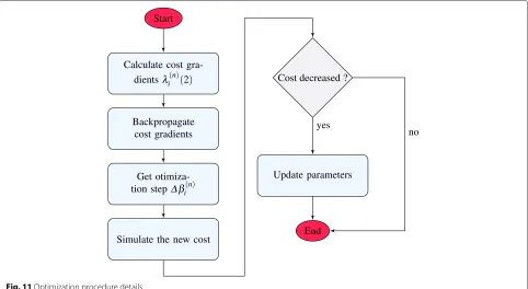
1.5.5 The optimization procedure

The optimization procedure described in this section integrates the analytical algorithm early detailed in Section 1.4. The working flow of the implemented opti-mization procedure is shown in Fig. 11. Firstly, the gra-dients of the cost function are calculated at the last layer

Table 2Simulation parameters

Parameter Value Description

K 4 Number of nodes in hidden and

exposed scenarios

63 Number of nodes in cellular scenario

NHnb 8 Number of hidden layer neurons in hidden and exposed scenarios

126 Number of hidden layer neurons in cellular scenario

μ 0.001 Learning rate

η 0.01,0.001 Optimization update rate

MaxEpochsnb 1000 Maximum number of training epochs

MSEdes 10−6 Desired mean squares error

FLdes 0.4 Desired fail limit (Mbps)

FNrdes 0.1 Desired fail number ratio

Offline DSenb 15 Offline data set entries number

TON 10s Data collection interval duration

MINPCSA −110 dBm Minimum PCS threshold value

MAXPCSA −60 dBm Maximum PCS threshold value

DEFPCSA −82 dBm Default PCS threshold value

MAXTPC 15 dBm Maximum transmit power value

MINTPC 0 dBm Minimum transmit power value

DEFTPC 6 dBm Default transmit power value

Load 20 Mbps Traffic load per device in hidden and exposed scenarios

4 Mbps Traffic load per device in cellular scenario

XT 20 Mbps Target throughput per device in hidden and exposed scenarios

4 Mbps Target throughput per device in cellular scenario

NSS 1 Number of spatial streams (antennas)

B 5 GHz Frequency band

BW 20 MHz Channel bandwidth

MCS MCS7 Modulation and coding scheme (no rate control)

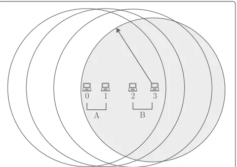
Fig. 12Hidden node scenario, illustration of the protection range at optimization round 0 (initial situation)

of the ANN as described in Eq. (12). Then, these val-ues are backpropagated through the ANN as described by Eq. (13). Consequently, the β values that will be used to adapt the MAC parameters are obtained as described by Eq. (14). In order to get the new optimized MAC parameters, each β value is added to its related old MAC parameter value as shown by Eq. (8). The update rateηdetermines how much the optimization process is aggressive in updating MAC parameters. Unless other-wise stated, the update rate ηis set to its default value indicated in Table 2.

Before sending the newly updated parametersβ_i(n+1)to their corresponding nodes, their performance is verified by simulating the resulting cost using the trained ANN. This step will prevent an unnecessary parameters update that may alter the current performance of the operational network. If the simulated cost is better than the cur-rent cost (cost decreases), an update message is sent back

to every registered node asking them to configure their transmission power and carrier sensing using the new optimized values. Otherwise, the nodes are not updated and they continue to use the old parametersβ_i(n)until the next optimization round.

1.6 Results and discussion

In this section, the performance of the proposed learning-based joint adaptation of PSCA and TPC is evaluated through extensive system level simulations. For these sim-ulations, we use the modified WLAN node model of OPNET 17.5 that implements the neural network solution as described earlier in this paper. The main parameters

of the simulation system are shown in Table 2. The men-tioned values are the initial values at the beginning of a simulation run. In order to assess the maximum amelio-ration that the proposed solution can achieve, the target throughout XT is set to the value of the traffic load. The performance of an ANN depends upon its general-ization capability. To avoid overtraining of the network, we stop the training procedure at the minimum of the validation error. The effect of some key parameters on the performance of the proposed solution is discussed and highlighted in this section. Firstly, we evaluate the performance of the proposed solution in mitigating hid-den and exposed node problems in two simple scenarios.

a

c

d

b

Fig. 15Exposed node scenario, illustration of the protection range at optimization round 0 (initial situation)

Then, we consider a more complex scenario that reflects a real-world high-density deployment and we evaluate our proposal in such challenging circumstances.

1.7 Hidden node scenario

We talk about a hidden node problem when a node that is not able to sense the signal transmitted by an another neighboring node (the hidden node) operating at the same channel, and hence, it assumes that the medium is free and transmits. The simultaneously transmitted signals inter-fere at the receiving node causing a failure in the reception process. As a solution to this problem, an exchange of request to send (RTS) and clear to send (CTS) frames is described in the IEEE 802.11 standard. However, as widely highlighted in the literature [31], the RTS/CTS mecha-nism introduces an important overhead and reduces the

Fig. 16Exposed node scenario, illustration of the protection range at optimization round 5

capacity of the network in terms of throughput since each node has to transmit the RTS and wait for the CTS response before any transmission. Furthermore, in spe-cific scenarios, this mechanism fails to eliminate hidden nodes [32]. In this study, we experiment the performance of our solution in solving the hidden node problem with-out using the RTS/CTS.

The topology used for this scenario consists of four nodes (two couples: coupleA includes node 0 and node 1 and couple Bincludes node 2 and node 3) placed as shown in Fig. 12. All these nodes are operating at the same frequency channel. Each node generates a saturated constant bit rate (CBR) traffic to the other node of the same couple. In this scenario, in order to reproduce the hidden node problem, the distances between the differ-ent nodes are configured in such a way that if two nodes belonging to different couples transmit simultaneously, both receiving nodes will not be able to receive the sig-nal of interest successfully. This means that coupleAand coupleBare sharing the total capacity of the network. Bas-ing on a simple simulation of a sBas-ingle transmitter-receiver couple, without any source of co-channel interference, the maximum capacity of a network using the default configurations is around 49 Mbps.

is fairly shared between the four nodes as shows the Jain’s fairness index in Fig. 14c.

As defined in Eq. (15),ηdetermines the aggressiveness of the optimization round update. The Fig. 14a shows that with a higherη, the cost is minimized with less optimiza-tion rounds. The same logic applies to the Jain’s fairness that reaches its maximum value after the first two opti-mization rounds for η = 0.01. It is worth mentioning that the cost function is not minimized to zero since the individual average throughput cannot reachXT (i.e., the target throughput). In fact, the maximum capacity of the network is attained before the satisfaction of the target throughput.

1.7.1 Exposed node scenario

In this scenario, we examine the ability of the proposed solution to mitigate the exposed node problem. The sce-nario topology shown in Fig. 15 consists of the same two couples of nodes used in the previous section but differ-ently configured to reproduce the exposed node problem. Here, the SINR values at a receiver node, in the presence of a simultaneous transmission with the other couple, always permit the receiver to decode successfully the signal of interest. However, the transmission power and carrier sensing are configured in such a way as to prohibit node 3 from transmitting when one of the nodes of coupleAis transmitting. Node 3 that belongs to coupleBis exposed

c

d

b

a

here to the transmissions of the nodes of couple A as illustrated in Fig. 15.

As in the previous scenario, we run the simulation for differentηvalues and we plot the resulting metrics over 5 optimization rounds in Fig. 17. At the initial situation (i.e., optimization round 0), the Jain’s fairness index in Fig. 17c shows clearly the impact of the exposed node problem. Node 3 is not able to gain access to the medium because it is exposed to the transmissions of the other couple. In this scenario, thanks to the initial configurations of the network topology, the maximum attainable capacity of the network is the aggregation of two transmitter-receiver couples (about 98 Mbps). This is due to the fact that relative interfering couples separation is sufficient for suc-cessful simultaneous transmissions. However, as clearly depicted in Fig. 17b, the aggregate throughput at the opti-mization round 0 is far away from the optimal value because node 3 is not able to initiate transmissions neither responding to the transmissions received from node 2.

Our proposed scheme is able to relieve the exposed node situation by decreasing the protection range around the exposed node (node 3) as illustrated in Fig. 16. This led, in this particular scenario, to a twofold increase in the aggregate throughput as shown in Fig. 17b at optimiza-tion round 5. Since the target throughputXTcan be easily

attained by the different nodes before the saturation point of the system, the cost function plotted in Fig. 17a is min-imized to zero at the last optimization round for all theη values.

1.7.2 High-density cellular deployment scenario

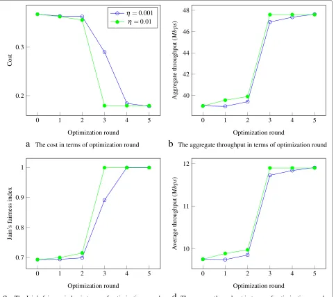
In this scenario, we consider a challenging super dense deployment. The definition of this scenario is based on the simulation scenarios defined by the IEEE 802.11ax TG [12]. An important real-world use case considered at the standardization TG is deploying Wi-Fi in a stadium which is characterized by very high numbers of APs and STAs [33]. In such deployments, the distance between two co-channel APs is below 25 m. The cellular scenario con-sidered for our evaluation is illustrated in Fig. 18. Each BSS is formed by an AP and eight associated STAs. With a frequency reuse equal to 3 and a cell radius of 7 m, the dis-tance between two co-channel APs is about 21 m. All the BSSs shown in the simulated scenario in Fig. 18 operate on the same frequency channel.

The obtained results are presented in Fig. 19. The first important observation when comparing to the results of the previous scenarios is that the system needs more opti-mization rounds to converge. This is normal since the scenario is more complex because of the much higher

a

c

d

b

Fig. 19The performance of the proposed optimization in cellular scenario.aThe cost in terms of optimization round.bThe aggregate throughput in terms of optimization round.cThe Jain’s fairness index in terms of optimization round.dThe average throughput in terms of optimization round

number of devices, and hence, the ANN has larger num-ber of neurons with 126 inputs and 63 outputs. Another observation is related to the Jain’s fairness index curve plotted in Fig. 19c. Contrary to the previous scenarios, this index does not reach its maximum value in the current scenario, meaning that not all the devices are achieving the same throughput.

In fact, this is due to the difference in throughput between uplink and downlink flows. The AP that is trans-mitting to eight STAs has almost the opportunity to access the medium as any other ordinary STA. Since the network is saturated, the share of airtime used by the AP to trans-mit data to one STA is much lower than that used by a

STA to send data to the AP. However, after the conver-gence of the adaptation, the fairness index is importantly enhanced (from≈0.5 at optimization round 0 to≈0.7 at the final round). This enhancement reflects the ability of the proposed adaptation to solve the exposed node sit-uations and increasing the spatial reuse between all the BSSs. This enhancement in spatial reuse is clearly seen in Fig. 19b, where the gain in aggregate throughput exceeds 45 %.

2 Conclusions

spatial reuse in high-density deployments by adapting the MAC layer protocols. While the control of the trans-mission power (i.e., TPC) has always been the chosen technique when targeting spatial reuse improvements (traditionally in cellular technologies), many researchers investigated the weakness points in TPC especially in deployments where the compliance of all the wireless devices is not always possible. Adapting the physical car-rier sensing is proposed in the IEEE 802.11ax task group where the preparations for the next WLAN standard are taking place. While, there are many more incentives behind preferring this adaptation over TPC, many con-tributions highlight some fairness issues especially when legacy devices are present in the network.

To overcome the previous problem, we exploit in this work a new solution for jointly optimizing the transmis-sion power and the physical carrier sensing. The main motivation of this joint solution is that the impact of one of these two key parameters on the performance of legacy devices is opposed to the other. While TPC mechanisms favor the legacies, the adaptation of the carrier sensing mechanism disfavors these devices. In this paper, we pro-posed a new learning-based mechanism using artificial neural networks that is able to optimally adapt the two mechanisms (TPC and PCSA) in order to increase spatial reuse and preserve fairness. This approach takes benefit from the capability of artificial neural networks to approx-imate complex functions in order to model the throughput performance in terms of MAC layer parameters. This allows an intelligent adaptation of these parameters that enhances the spatial reuse in dense deployments. We showed through extensive simulations that our proposal is capable of resolving hidden and exposed node problems and hence leveraging the aggregate throughput in high-density deployments while enhancing the fairness among all the nodes.

Furthermore, this solution could be used to optimize other important parameters in the future IEEE 802.11ax WLANs such as the length of the transmit opportu-nity (TxOP). Future centralized deployments could ben-efit directly from this new approach to achieve better QoE. This would allow the integration of high efficiency WLANs in mobile cellular networks for traffic offloading.

Competing interests

The authors declare that they have no competing interests.

Author details

1_{Orange, 4 Rue de Clos Courtel, 35510 Cesson-Sevigne, France.}2_{Intel, 2111 NE} 21st Avenue, Hillsboro, OR, USA.3_{Institute of Electronics and}

Telecommunications of Rennes (IETR)—Institut National des Sciences Appliquées (INSA) de Rennes, 20 Avenue des Buttes de Coesmes, 35708 Rennes, France.

Received: 27 October 2015 Accepted: 7 May 2016

References

1. IEEE Std 802.11-2012 (Revision of IEEE Std 802.11-2007),IEEE Standard for Information technology—Telecommunications and information exchange between systems local and metropolitan area networks— specific requirements. Part 11: wireless LAN medium access control (MAC) and physical layer (PHY) specifications. (IEEE, 2012), pp. 1–2793

2. A Baid, D Raychaudhuri, Understanding channel selection dynamics in dense Wi-Fi networks. IEEE Commun. Mag.53, 110–117 (2015) 3. iPass Wi-Fi service provider, The global public Wi-Fi network grows to 50

million worldwide Wi-Fi hotspots. http://www.ipass.com/press-releases/ the-global-public-wi-fi-network-grows-to-50-million-worldwide-wi-fi-hotspots

4. IEEE 802.11 High efficiency wireless local area networks (HEW) study group. http://www.ieee802.org/11/Reports/hew_update.htm 5. IEEE 802.11ax task group for high efficiency WLAN (HEW). http://www.

ieee802.org/11/Reports/tgax_update.htm

6. D-J Deng, C-H Ke, H-H Chen, Y-M Huang, Contention window optimization for. IEEE 802.11 DCF access control. IEEE Trans. Wirel. Commun.7, 5129–5135 (2008)

7. B Li, Q Qu, Z Yan, M Yang, inProceedings of the IEEE Wireless Communications and Networking Conference Workshops. Survey on OFDMA based MAC protocols for the next generation WLAN, WCNC ’15 (IEEE, 2015), pp. 131–135

8. A Ben Makhlouf, M Hamdi, Dynamic multiuser sub-channels allocation and real-time aggregation model for IEEE 802.11 WLANs. IEEE Trans. Wirel. Commun.13, 6015–6026 (2014)

9. I Jamil, L Cariou, inIEEE 802.11ax: 802.11-14/0523r0. MAC simulation results for dynamic sensitivity control (DSC-CCA adaptation) and transmit power control (TPC) (IEEE, 2014)

10. I Jamil, L Cariou, inIEEE 802.11ax: 802.11-14/1207r1. OBSS reuse mechanism which preserves fairness (IEEE, 2014)

11. I Jamil, L Cariou, J-F Helard, inProceedings of the IEEE International Conference on Communication Workshop, ICC ’15. Preserving fairness in super dense WLANs, (2015), pp. 2276–2281

12. S Merlin, et al, inIEEE 802.11ax: 802.11-14/0980r14. TGax simulation scenarios (IEEE, 2015)

13. SS Haykin, inNeural Networks and Learning Machines. Number v. 10 in neural networks and learning machines (Prentice Hall, 2009)

14. RP Lippmann, Pattern classification using neural networks. IEEE Commun. Mag.27, 47–50 (1989)

15. Y-K Park, G Lee, Applications of neural networks in high-speed communication networks. IEEE Commun. Mag.33, 68–74 (1995) 16. C Wang, J Hsu, K Liang, T Tai, inProceedings of the 3rd IEEE International

Conference on Computer Science and Information Technology, volume 4 of ICCSIT ’10. Application of neural networks on rate adaptation in IEEE 802.11 WLAN with multiples nodes (IEEE, 2010), pp. 425–430

17. C-L Chen, inProceedings of the 16th International Conference on Computer Communications and Networks, ICCCN ’07. IEEE 802.11e EDCA QoS provisioning with dynamic fuzzy control and cross-layer interface (IEEE, 2007), pp. 766–771

18. P Lin, T Lin, Machine-learning-based adaptive approach for frame-size optimization in wireless LAN environments. IEEE Trans. Veh. Technol.58, 5060–5073 (2009)

19. H Luo, NK Shankaranarayanan, inProceedings of the IEEE International Conference on Acoustics, Speech, and Signal Processing, volume 5 of ICASSP ’04. A distributed dynamic channel allocation technique for throughput improvement in a dense WLAN environment, vol. 5, (2004), pp. V–345–8 20. P Gogoi, KK Sarma, inProceedings of the International Conference on

Communications, Devices and Intelligent Systems, CODIS ’12. Hybrid channel estimation scheme for IEEE 802.11n-based STBC MIMO system (IEEE, 2012), pp. 49–52

21. H Zhang, X Shi, inProceedings of the 10th World Congress on Intelligent Control and Automation, WCICA ’12. A new indoor location technology using back propagation neural network to fit the RSSI-d curve (IEEE, 2012), pp. 80–83

23. V Shah, S Krishnamurthy, inProceedings of the 25th IEEE International Conference on Distributed Computing Systems, ICDCS ’05. Handling asymmetry in power heterogeneous ad hoc networks: a cross layer approach (IEEE Computer Society, 2005), pp. 749–759

24. A Pires, J Rezende, C Cordeiro, inChallenges in Ad Hoc Networking. Protecting transmissions when using power control on 802.11 ad hoc networks (Springer US, Boston, 2006), pp. 41–50. IFIP International Federation for Information Processing

25. B Radunovi´c, R Chandra, D Gunawardena, inProceedings of the 8th International Conference on Emerging Networking Experiments and Technologies, CoNEXT ’12. Weeble: enabling low-power nodes to coexist with high-power nodes in white space networks (ACM, New-York, 2012), pp. 205–216

26. M van der Schaar, N Sai Shankar, Cross-layer wireless multimedia transmission: challenges, principles, and new paradigms. IEEE Wirel. Commun.12, 50–58 (2005)

27. Neural Netw. Multilayer feedforward networks are universal approximators.2, 359–366 (1989)

28. IEEE Std 802.11e-2005 (Amendment to IEEE Std 802.11, 1999 Ed1ition (Reaff 2003)),IEEE Standard for Information technology—Local and metropolitan area networks—specific requirements—part 11: wireless LAN medium access control (MAC) and physical layer (PHY)

specifications—amendment 8: medium access control (MAC) quality of service enhancements. (IEEE, 2005), pp. 1–212

29. C Wang, P-C Lin, T Lin, A cross-layer adaptation scheme for improving IEEE 802.11e QoS by learning. IEEE Trans. Neural Netw.17, 1661–1665 (2006) 30. R Jain, D-M Chiu, WR Hawe,A quantitative measure of fairness and

discrimination for resource allocation in shared computer system, (1984). Technical Report, Eastern Research Laboratory, Digital Equipment Corporation Hudson, MA, DEC-TR-301

31. JL Sobrinho, R de Haan, JM Brazio, inProceedings of the IEEE Wireless Communications and Networking Conference, volume 1 of WCNC ’05. Why RTS-CTS is not your ideal wireless LAN multiple access protocol (IEEE, 2005), pp. 81–87

32. K Xu, M Gerla, S Bae, inProceedings of the IEEE Global Telecommunications Conference, volume 1 of GLOBECOM ’02. How effective is the IEEE 802.11 RTS/CTS handshake in ad hoc networks (IEEE, 2002), pp. 72–76 33. L Cariou, inIEEE 802.11 HEW: 11-13/0657r3. HEW SG usage models and

requirements—liaison with WFA (IEEE, 2013)

Submit your manuscript to a

journal and benefi t from:

7Convenient online submission

7 Rigorous peer review

7Immediate publication on acceptance

7 Open access: articles freely available online

7High visibility within the fi eld

7 Retaining the copyright to your article