Volume 2010, Article ID 270894,8pages doi:10.1155/2010/270894
Research Article
Distributed Transmit Beamforming without Phase Feedback
Chen Wang, Qinye Yin, Jingjing Zhang, Bo Hao, and Wei Li
Ministry of Education Key Laboratory for Intelligent Networks and Network Security, Xi’an Jiaotong University, 28 West Xianning Road, Xi’an, Shaanxi 710049, China
Correspondence should be addressed to Chen Wang,[email protected]
Received 30 October 2009; Accepted 30 March 2010
Academic Editor: Xinbing Wang
Copyright © 2010 Chen Wang et al. This is an open access article distributed under the Creative Commons Attribution License, which permits unrestricted use, distribution, and reproduction in any medium, provided the original work is properly cited.
Phase feedback and adjustment between wireless nodes greatly reduce the power efficiency of distributed beamforming. In this paper, we propose a distributed transmit beamforming method without any phase feedback between nodes. The concept of our approach is to have the received signals retrace their ways, so that the phase offset of the forward path compensates that of the backward path; as a result, signals from different nodes in-phase combine at the destination. Therefore, the received power or the communication range is increased. In order to implement the concept of “retracement”, we also propose a transceiver prototype which is based on the Direct Digital Synthesis technique. Experimental and simulation results validate the effectiveness of our approach.
1. Introduction
Long-range communication is a typical issue in Wireless Sensor Networks (WSNs). Direct transmission from a sensor node to a distant destination node requires high transmit power, which is not feasible for WSNs because of the size and power supply constrains on wireless sensor nodes. Therefore, it turns to the multihop fashion when the destination is located beyond one-hop coverage. However, in some applications, there is no relay node between the source and destination. For example, an Unmanned Arial Vehicle (UAV) collects sensor information from a cluster of nodes
deployed in a certain area as shown in Figure 1. Due to
some safety considerations the UAV cannot fly low enough to be within the single node coverage. Therefore, cooperation among the nodes becomes one possible approach. However,
the popular distributed space-time code [1] and
space-frequency code approaches [2] are mainly focused on the
enhancement of reliability but not this kind of large-scale fading occurring over long distances. Another approach exploiting multiple antennas is the smart antenna system (SAS), which reallocates the energy in space through the coherent combination of radio frequency (RF) signals and forms a beam at the destination. As a result, the commu-nication range increases without any power enhancement
on each antenna. The concept of SAS can be utilized in WSNs where coherent signals transmitting from multiple nodes constructively combine at the destination so that
the received power is enhanced [3, 4]. For the case of N
collaborative nodes, the received power gain is N2 which
means anN-times larger communication range for free space
propagation.
Although distributed beamforming promises many advantages, it faces many practical challenges too. The first challenge is the frequency synchronization between nodes
[5]. The traditional SAS does not suffer from this problem
because all antennas share a common local oscillator, so the signals are coherent in nature. However, in distributed beamforming system, nodes have their independent
oscilla-tors; so there are frequency offsets between them. In order
to synchronize the frequency, one node (e.g., destination) broadcasts a high-power reference signal to each source node and source node adjusts its frequency of oscillator to that of
[6–8]. Second, phase synchronization is also needed so that
the signals are constructively combined at the destination, or they will cancel out each other. It should be noted that our phase synchronization means that signals have the same phase at the destination, not at the sources. The work in
[9] divides the phase synchronization methods into
the phases of nodes one by one [10] or adjust the phases
of all nodes simultaneously [11, 12]. However, they all
require the feed back of phase adjustment information from
a certain node. The work in [13] proposes a scheme that
does not require any phase precompensation. Instead, the destination node broadcasts a node selection vector to the pool of available source nodes to opportunistically select a subset of nodes whose transmitting signals combine in a quasi-in-phase manner at the destination. However, this node selection vector is also a feedback. Moreover, the energy on all the nodes cannot be fully exploited because it only selects a subset of available nodes. In one word, the
feedback procedure decreases the efficiency of distributed
beamforming.
This paper proposes a distributed transmit beamforming
scheme which eliminates the inefficient feedback procedure.
It utilizes the reciprocity of the signal propagation in space. By reversing the transmit sequence, the transmitting signals of the collaborative nodes “retrace their ways”, and the phase shifts from the forward and backward path are automatically cancelled out so that they are in-phase combined at the destination. The collaborative nodes synchronize to the reference signal simultaneously and independently. The complexity of the network does not increase with the number of collaborative nodes, which fits the massively deployed WSNs.
The rest of the paper is organized as follows.Section 2
describes the system model for distributed beamforming. Then, we introduce our proposed beamforming method
with discussion on the implementation aspect inSection 3.
Section 4simulates the influence of frequency and phase syn-chronization errors on performance. A hardware experiment
is described inSection 5, which demonstrates the validity of
distributed beamforming. Finally, the conclusions are given inSection 6.
2. Models and Main Assumptions
2.1. Network Structure. Nodes in the system are classified into two kinds: source node and destination node. A source node is typically characterized by low-cost, small size, resource-constrained, power limited, and so forth, while a destination node usually has more resources, adequate power supply, and higher transmission power so that all the source nodes could receive its signal. In WSNs, the wireless sensor nodes (source nodes) usually need to send their gathered messages to the data sink node; so the destination is also referred to as the sink node. Source collects data and transmits them back to the destination for further data analysis. However, a single source node constrained by node transmit power cannot directly send the information back to the destination node by single-hop. In this case, the source nodes perform distributed beamforming at the distant destination, making the signals in-phase combined there so that information is delivered by just one hop.
2.2. Signal Model. We adopt the free-space signal propaga-tion model with assumppropaga-tion of line-of-sight (LOS) channels
Coverage of
Figure1: Single node cannot communicate with UAV directly.
to simplify our discussion. We first consider the change of the signal between a transmitter and a receiver during the communication process. The transmitting signal is
s(t)=ejωt. (1)
The received signal is the attenuated transmitted signal with
time delayτ, that is,
r(t)=gs(t−τ), (2)
wheregis the amplitude gain in free-space propagation,g =
λ/4πd,λis the signal wavelength,dis the distance between
the nodes,τ is the propagation delay, andτ =d/c,cis the
speed of light. For a narrow band signal, say sinusoidal signal, the time delay represents phase shift, that is,
r(t)=ge−jωτs(t). (3)
Distributed beamforming at the destination node is to make the transmitting signals of multiple nodes have the same phase at the destination, that is, in-phase combination.
3. Beamforming without Phase Feedback
For a cluster of densely deployed sources, their gathered information is often highly correlated. So usually the data are firstly fused among the sources, and then sent back to the destination. Assume that before beamforming, all collaborative nodes have already obtained the common
message m(t) which is to be transmitted. When adopting
time division duplex (TDD) mode, our approach can be divided into two time slots: synchronization time slot and beamforming time slot. In synchronization slot, the signal of each source node will be synchronized to the reference signal broadcasted by the destination node; in beamforming time slot, all the transmitting signals of source nodes are coherently combined at the destination node. Because there is no reference signal for sources to synchronize in beamforming slot, two slots repeat alternately as shown in Figure 2. Obviously, the synchronization time slot does
Synchronization Beamforming Synchronization Beamforming · · ·
Figure2: Time slots structure for TDD mode.
that it is more important to successfully send the valuable message back to the sink node than to transmit more
efficiently in this scenario.
3.1. Synchronization Time Slot. In this time slot, the desti-nation node broadcasts a high-power reference signal, say sinusoidal signal:
sd(t)=ejωt. (4)
According to (3), the signal received at the ith source after
delay and attenuation is
ri(t)=gie−jωτiejωt, (5)
where gi and τi are channel gain and propagation delay
between theith source and the destination, respectively.
Every source node continuously adjusts its local oscillator
signal si(t) within the specified time slot, making its
fre-quency and phase synchronize to those of the received signal. That is:
si(t)=ri(t)
gi . (6)
There are many ways for frequency and phase
synchroniza-tion. Readers may refer to [14,15], and so forth.
3.2. Beamforming Time Slot. When frequency and phase synchronization is completed, the adjusted local oscillator signal will be output in time reverse order in beamforming slot, that is,
si(t)=si(−t)= ri(−t)
gi , (7)
and the messagem(t) will be modulated to the carriersi(t).
After transmission, the signals from N sources combine at
the destination node:
From (9) we note that the phase shift between the source
and the destination has been cancelled through the reverse
transmission of signals. For the common messagem(t), due
to the low data rate in sensor networks, we consider m(t)
as a narrowband signal compared with the carrier ω, then
m(t−τi)≈m(t). The received signal can be rewritten as
So transmitted signals in-phase combine at the destination node, and the received amplitude is the summation of the
amplitudes ofNnodes.
Due to the long distance between the source node and
the destination node, the channel gaingibetween each source
and the destination can be regarded as the same, namely,gi=
g. Then the received signal power is
Pr(t)= |rd(t)|2=
Ngm(t)2=N2gm(t)2. (11) Compared with a single-node case, there is an enhancement
of 20 log10NdB in received power.
Note that for non-LOS environment, as long as the backward propagation environment is consistent with the forward one, the above method can also result in in-phase combination at the destination. Theoretically, the scheme of the proposed method is feasible if the synchronization process can catch up with the change of wireless channels. As far as our following experiment concerns, we just carried out experiments in static environment.
3.3. Discussion on Design and Implementation of Source Node. One key point of the proposed method lies in the transmission of the time-reversed signal from source node. However, the local oscillator of the RF transceiver usually
has a relatively high frequency. It is very difficult to control
its frequency and phase directly, especially for the low-cost wireless sensor nodes. We adopt the direct-conversion architecture (zero-IF) transceiver which is popular in low-cost applications. Based on this architecture, we set another “oscillator” in the baseband to control frequency and phase indirectly so that the upconverted RF signal is coherent. For
digital transceivers it can be implemented as inFigure 3.
The baseband oscillator can be implemented with a direct digital synthesizer (DDS) which continuously generates complex sinusoid signal whose frequency and phase can be
precisely controlled by its phase increment and phase offset
register, respectively. In the synchronization slot, the sources work in receive mode and downconvert the sinusoidal signal broadcast from the destination, sample and convert to digital signal with ADCs, and then send the baseband IQ signal to the synchronization module. By comparing the received signal with the output of the baseband oscillator, synchronization module calculates the frequency and phase
offset and adjusts those of the baseband oscillator so as to
make them synchronized [14, 15]. In this case, frequency
synchronization is achieved by adjusting the phase increment of the DDS, while phase synchronization is achieved by
adjusting the phase offset register of the DDS. The
synchro-nization process can be done in iterative approach so as to obtain an accurate result by simple algorithm. Due to the limitation of the paper, we will describe the specific details of the implementation in our future papers. In beamforming slot, the sources switch to transmit mode with the baseband oscillator running continuously but in reverse sequence. To achieve this, the only change of the transceiver is the sign of phase increment, which turns the phase accumulator in the synchronization time slot into a phase decreaser in
Rx
Figure3: The transceiver uses a baseband oscillator to control the RF signal indirectly.
Beamforming time slot (phase decreases) Synchronization time slot (phase increases)
End of
Figure4: Output waveform of DDS in beamforming time slot is in reverse time sequence to that in synchronization time slot.
The message m(t) is modulated by the reversed baseband
oscillator, converted to analogue signal with DACs, and finally upconverted to RF signal.
4. Simulations
As aforementioned, during the synchronization slot, sources should synchronize frequency and phase in order to make the local signal have the same phase and frequency as that of the received signal. However, in reality, absolute frequency and phase coherence is impossible, because of the noise and the instability of the crystal oscillator, and so forth. Suppose
that the transmit signal of theith source has frequency error
Δfiand phase errorθi,e, then according to (10), the received
signal at the destination is
rd(t)=m(t)e−jωt
which indicates that the amplitude of the received signal is no longer the sum of signals’ amplitudes. The following
simulation shows the effect of frequency and phase error on
beamforming performance.
4.1. Effect of Phase Error on Performance. Suppose that there is only phase error but no frequency error, and then the power of the received signal at the destination node is
Pr(t)=
It shows that transmit signals do not completely in-phase combine at the destination node, which reduces the ampli-tude of the received signal.
To simplify our analysis, suppose that signal transmitted from each source has the same power at the destination node,
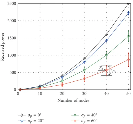
Es 2
Figure 5: Relation between received power and the number of nodes under different phase errors.
Gaussian random variableθi,e∼N(0,σ2p).Figure 5illustrates
the relationship between the number of collaborative nodes
and the received power under different phase errors. The
average (Es) and the standard deviation (σs) of the received
power are obtained after 5000 trials of simulation.
As is shown in Figure 5, the average received power
increases with node number. However, it is not proportional
to N2, because of the existence of phase error. With the
phase error increasing, the average of the received power falls while its variance rises. Nevertheless, we note that the beamforming is not sensitive to phase error; when the variance of phase error is 40 degree, the received power could still reach 60% of the ideal value.
4.2. Effect of Frequency Error on Performance. Because phase is the integration of frequency over time, a small frequency synchronization error can result in a large phase drift. Even though all the signals are synchronized at the beginning, they are not in-phase any more as time goes by, which causes the received power at the destination to fluctuate with time.
The bigger frequency offset is, the faster the received power
changes. Here we define the coherent collaborative timeT3 dB
as the time duration in which the received power drops from its peak to its half level (for two-node case the half power is 3 dB lower than its peak; so we denote it with subscript 3 dB):
T3 dB=min
t|Pr(t)<Pr,max
2 . (14)
It indicates the time duration in which distributed
beam-forming with frequency offset could perform effectively.
Figure 6 shows the relation between T3 dB and frequency
errors with different number of collaborative nodes. In the
simulation, we suppose that the phases of all the sensors are synchronized at the beginning of the beamforming, namely,
104
103
102
101
Standard deviation of frequency error (Hz)
N=2
Figure 6: Relation betweenT3 dBand frequency synchronization
error with different number of nodes.
θi,e =0, for alliin (12), and frequency error is modeled as a
zero-mean Gaussian random variableΔfi∼N(0,σ2
f).
According toFigure 6,T3 dBdecreases as frequency offset
increases. Besides, the number of nodes also affects T3 dB.
When the number of sensors is small (N < 5), T3 dB falls
rapidly asNincreases.T3 dBdoes not change greatly any more
withNforN >7. When the standard deviation of frequency
errors among sensors is 100 Hz, T3 dB is millisecond order
of magnitude, which satisfies the demands of most of the communication protocols (e.g., the longest packet duration is 4.256 ms for IEEE 802.15.4).
5. Hardware Experiment
5.1. Verification of Coherent Transmission Using Independent Wireless Nodes. The following experiment demonstrates the feasibility of the coherent superposition of two indepen-dent sensors. The complexity and time-variance of wireless
channel will affect the accuracy of measurement result.
In order to analyse with an accurate measurement, some devices such as the power combiner are used to simulate the superposition of the RF signal while excluding the impact of the time-varying wireless environment. The experiment
setup is shown inFigure 7. The RF signal which is combined
from two transmitted signals by a combiner is input to a spectrum analyzer. The spectrum analyzer is set to Zero-Span mode in order to observe the change of the combined signal’s power versus time. By observing the change of the signal power, we could obtain the quantitative indicator of the power enhancement for coherent combination.
We set the two nodes to the same frequency and phase by manually adjusting the control words of DDS. In the experiment, each sensor has an independent local
Node number 2 Combiner
Coaxial cables
Spectrum analyzer Node number 1
Figure7: Experiment setup of the test platform.
adjusting DDS output frequency and phase of one sensor,
the frequency and phase offsets are compensated manually.
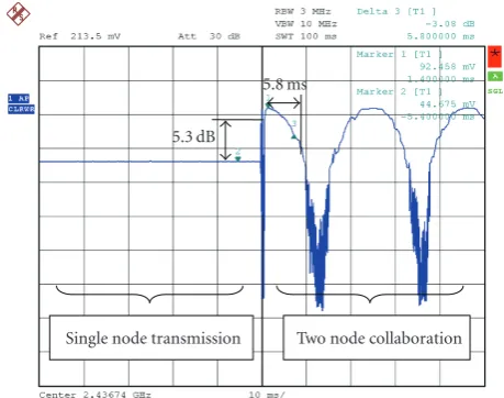
Figure 8is the captured result from the spectrum analyzer. In the experiment, the signal amplitude of nodes no. 1 and no. 2 is 55.8 mV and 44.6 mV (Marker 2), respectively, and the maximum signal amplitude after combination is 92.4 mV (Marker 1); so the coherent collaboration achieves 92% of its ideal value. This equals to 5.3 dB power gain compared with single node transmission (the theoretical gain is 6 dB for two nodes transmission). From the experiment, we also see that the compensation at a certain time will be gradually invalidated with time because of the short-term instability of the oscillator’s output frequency. However, this fluctuation in oscillator’s frequency is slow and we just adopt some low cost oscillators whose frequency stability is above 25 ppm. Using TCXO (Temperature Compensated Crystal Oscillator with frequency stability typically lower than 1 ppm) will further
slow this change. The measurement result shown inFigure 8
indicates thatT3 dBis 5.8 ms (Delta Marker 3 with reference
to Marker 1) and the period of the received signal’s power is about 20 ms which equals to 50 Hz of the frequency error.
5.2. Experiment of the Proposed Method. The above section has already shown the feasibility of two independent nodes beamforming in real system. In this section, we implement the proposed method on hardware system and show its high
beamforming efficiency from our experiment result. The test
system platform is illustrated inFigure 9.
In order to simulate the amplitude attenuation in real space propagation, we add an attenuator of 40 dB at the radio front end of the destination node. The reference signal trans-mitted by the destination node is distributed to two source nodes through Combiner/Splitter 1 in synchronization time slot. In beamforming time slot, the transmitted signals from two sources are first combined by Combiner/Splitter 1, and then split to the destination node and the spectrum analyzer by Combiner/Splitter 2. The measurement results from the
spectrum analyzer are shown inTable 1. In this experiment,
Single node transmission Two node collaboration 5.3 dB
5.8 ms
Figure8: The measured received power for two-node collabora-tion.
Source number 1
Destination
Combiner/splitter 1 Combiner/splitter 2
Attenuator
Coaxial cables
Spectrum analyzer Source number 2
Figure9: Experiment setup for the proposed method.
Table1: Experiment results.
Transmitting node(s) Received power of spectrum analyzer Source no. 1 −5.11 dBm (124.16 mV) Source no. 2 −3.92 dBm (142.39 mV) Source no. 1 and no. 2 1.02 dBm (251.47 mV)
the time durations of synchronization and beamforming are set to around 3 ms.
Ideally, the maximum beamforming power of Source no. 1 and no. 2 can be 266.55 mV, while the actual
measured result is 251.47 mV. The beamforming efficiency
is 94.3% (equivalent beamforming gain is 5.5 dB with 6 dB for ideal situation) compared with the experiment result of
beamforming efficiency 90.3% (5.1 dB beamforming gain) in
[9].
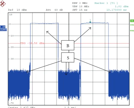
B
S
Figure 10: Only one source node is switched on. Note: that S represents the synchronization time slot during which sources are in receive mode and B represents the beamforming time slot.
B
S
Figure11: Received power waveform in time-domain when two sources beamform at the destination.
inFigure 10. A similar result is obtained when only Source
no. 2 transmits, except with different amplitude.
When the two sources work at the same time, their signals combine in-phase at the destination according to
the proposed beamforming technique.Figure 11shows the
received power of beamforming signal.
We can see from Figure 11 that the received power is
relatively high during the entire beamforming slot, which
indicates that the coherent collaborative timeT3 dBis longer
than 3 ms. Because the two sources perform good frequency-phase synchronization, there is just a small frequency dif-ference which has a very limited influence on beamforming result during the 3 ms. However, when we increase the noise or decrease the transmit power of the reference signal, the performance of the synchronization deteriorates, which
B
S
Figure12: A bigger frequency difference of source nodes leads to a shorter beamforming coherent collaborative time.
results in a short coherent collaborative time as shown in
Figure 12.
6. Conclusion
In this paper, we present a distributed transmit beamforming method, whose most distinct characteristic is to make the signals “retrace their ways to the destination”. Consequently, it avoids the complicated feedback adjustment process. In addition, the simulation shows that an increase in the number of collaborative nodes, the phase error, or the frequency synchronization error results in decrease of the
beamforming efficiency. Moreover, a transceiver reference
prototype based on DDS is introduced, and some hardware experiments based on this architecture have been conducted. Experiment result shows the feasibility of coherent trans-mission among independent wireless nodes. In the case of two nodes beamforming using the proposed method, the received signal power achieves 92% of its ideal value, which is 5.3 dB higher compared with signal node transmission.
Acknowledgments
This work is supported in part by the National Natural Science Foundation of China (NSFC) under Grant no. 60772095 and the Funds for Creative Research Groups of China under Grant no. 60921003.
References
[1] J. N. Laneman and G. W. Wornell, “Distributed space-time-coded protocols for exploiting cooperative diversity in wireless networks,”IEEE Transactions on Information Theory, vol. 49, no. 10, pp. 2415–2425, 2003.
IEEE Transactions on Vehicular Technology, vol. 58, no. 1, pp. 207–217, 2009.
[3] D. R. Brown III and H. V. Poor, “Time-slotted round-trip carrier synchronization for distributed beamforming,”IEEE Transactions on Signal Processing, vol. 56, no. 11, pp. 5630– 5643, 2008.
[4] D. R. Brown III, G. B. Prince, and J. A. McNeill, “A method for carrier frequency and phase synchronization of two autonomous cooperative transmitters,” inProceedings of the 6th IEEE Workshop on Signal Processing Advances in Wireless Communications (SPAWC ’05), pp. 260–264, June 2005. [5] I. Ozil and D. R. Brown III, “Time-slotted round-trip
carrier synchronization,” inProceedings of the 41st Asilomar Conference on Signals, Systems and Computers (ACSSC ’07), pp. 1781–1785, Pacific Grove, Calif, USA, November 2007. [6] G. Barriac, R. Mudumbai, and U. Madhow, “Distributed
beamforming for information transfer in sensor networks,” in
Proceedings of the 3rd International Symposium on Information Processing in Sensor Networks (IPSN ’04), pp. 81–88, Berkeley, Calif, USA, April 2004.
[7] R. Mudumbai, D. R. Brown, U. Madhow, and H. V. Poor, “Distributed transmit beamforming: challenges and recent progress,”IEEE Communications Magazine, vol. 47, no. 2, pp. 102–110, 2009.
[8] R. Mudumbai, G. Barriac, and U. Madhow, “On the feasibility of distributed beamforming in wireless networks,” IEEE Transactions on Wireless Communications, vol. 6, no. 5, pp. 1754–1763, 2007.
[9] R. Mudumbai, B. Wild, U. Madhow, and K. Ramchandran, “Distributed beamforming using 1 bit feedback: from concept to realization,” inProceedings of the 44th Allerton Conference on Communication Control and Computing, Monticello, Ill, USA, September 2006.
[10] P. Jeevan, S. Pollin, A. Bahai, and P. P. Varaiya, “Pairwise algorithm for distributed transmit beamforming,” in Proceed-ings of the IEEE International Conference on Communications (ICC ’08), pp. 4245–4249, Beijing, China, May 2008. [11] M. Pun, D. Brown, and H. Poor, “Opportunistic collaborative
beamforming with one-bit feedback,” IEEE Transactions on Wireless Communications, vol. 8, no. 5, pp. 2629–2641, 2009. [12] M. F. A. Ahmed and S. A. Vorobyov, “Collaborative
beam-forming for wireless sensor networks with Gaussian dis-tributed sensor nodes,”IEEE Transactions on Wireless Commu-nications, vol. 8, no. 2, pp. 638–643, 2009.
[13] H. Ochiai, P. Mitran, H. V. Poor, and V. Tarokh, “Collaborative beamforming for distributed wireless ad hoc sensor networks,”
IEEE Transactions on Signal Processing, vol. 53, no. 11, pp. 4110–4124, 2005.
[14] D. C. Rife and R. R. Boorstyn, “Single-tone parameter esti-mation from discrete-time observations,”IEEE Transactions on Information Theory, vol. 20, no. 5, pp. 591–598, 1974. [15] S. A. Tretter, “Estimating the frequency of a noisy sinusoid by