A Spectroscopic Study of
Planetary Nebulae in the
Magellanic Clouds
A thesis suhmitted hy
David
James
Monkto the
University of London
lor the degree 01 Doctor 01 Philosophy
On the advice of the examiners.
Page 36, paragraph 3, line 5. 'This additional.. ... image tube chain.'. Replace
with new sentence 'This additional reduction in flux at short wavelengths is attributable
to the narrower slit used for the medium resolution spectra.'.
Page 61, paragraph 3, line 1. Replace 'for each level' with 'for each transition'. Page 67, Section 3.3. Add 'Fo\1owing the work of Peimbert and Torres-Peimbert
(1971) the effects of co\1isional excitations on He I line intensities are ignored.'.
Page 120, paragraph 2, line 6. Replace 'If a particular model predicts a larger value for this ratio than is observed,' with 'The predicted ratio assumes that all photons
shortward of 504
A
are absorbed by helium. However, if the He+ /H+ ratio derived from the observations is equal to 0.1 or larger,'.Chapter 5 (pp 132-150).
The unreliable nature of the [N 11](6548+6585)/5755
A
flux ratio as an electron temperature diagnostic is clearly seen in Fig. 5.4, and is really more suitable, in this case, as an electron density diagnostic. In fact its shorter wavelength range makes itless sensitive to any errors in the reddening correction and therefore a better density
diagnostic than the [011]3727/7325
A
flux ratio. A guide to the electron temperature can be obtained from the [0111](4959+5007)/4363A
flux ratio, where the upper limit to [0 III] 4363A
is used to obtain a T,. upper limit. The derived value of this ratio (>95.3) combined with the [N II] ratio yields an electron temperature of <12100 K andan electron density of> 5.3 x 104 cm-3•
The ionic and elemental abundances of LMC N25 have been recalculated for this
electron temperature and density, and for an electron temperature of 10000 K with
It should be noted that the elemental abundances of LMC N25 are increased
signif-icantly at the lower T, values, particularly the oxygen abundance (1 - 4 x 10⁻⁴
), which
is within the range found about the mean LMC PN oxygen abundance (3.1 x 10⁻⁴ ).
LMC N25 is therefore probably a low-excitation, normal abundance nebula and not
a low-oxygen nebula, and the above analysis also makes the 'low-oxygen' description of
the other LMC and SMC PN in Table 3.9 doubtful. For this reason the electron
temper-atures for these objects (given in Table 2.1) have been bracketed and their abundances
(Tables 3.4,3.5,3.6 and 3.9) have been flagged as uncertain (::). It is also noted that the
discussion of the elemental abundances of LMC N25 on page 142 is now irrelevant.
The lower electron temperature for LMC N25 also leads to a lower nebular
contin-uum (decreases of 22% and 43% in the nebular contincontin-uum at 4500 A for Tr equals 12100 K and 10000 K respectively) and therefore a slightly higher stellar continuum (the
neb-ular continuum level at 4500
A
being 32% and 24% of the total continuum for Tp equals 12100 K and 10000 K respectively). The best fit model to this new stellar continuumlevel is a Mihalas 40000 K, log g 3.5, model, giving a stellar luminosity of 12000
±
1000 LG, a core mass of 0.685±
0.015 MG, a stellar radius of 2.3±
0.1 RG, and a predictedlog g of 3.5
±
0.1. This new Zanstra temperature of 40000±
5000 K could be consistent with a significant neutral helium abundance if it was at the lower end of its allowedrange. The new 0+ /0 ratio (0.85 - 0.90) does indicate a large neutral helium content (Torres-Peimbert and Peimbert, 1977). Similarly, the upper limit on the [Ne IIIj3868
A
flux of <2.3 is probably inconsistent with a high temperature central star. It should be noted that in this effective temperature range the derived stellar luminosity dependsmainly on the absolute nebular H,8 flux, which for LMC N25 is significantly larger than
the average.
Ion -\( A )
N+ 6548+6584
0" 6300
0+ 3727
0+ 7325
0++ 5007+4959
Ne++ 3868
s+ 4068+4076
s++ 6312
Ar++ 7135
n (tntt)
n(H+)
T.=12100 K
1.04 x 10-;
3.11 x 10⁻⁶
9.41 x 10-(. 6.49 x 10-(' 1.41 x 10-;
< 9.22 x 10⁻⁷
1.69 x 10⁻⁷ 9.10 x 10⁻⁷
1.29 x 10⁻⁷
n(i.ln)
,o(H+ )
T.=10000 K
2.30 x 10⁻⁶
6.03 X 10⁻⁶
3.68 X 10⁻⁴
1.77 X 10⁻⁴
2.75 x 10-; < 1.88 X IO-G
2.59 X 10⁻⁷
1.73 X 10-(;
1.97 X 10⁻⁷
Element N 0 Ne S Ar Element.al
T. =12100 K
1.23 X 10⁻⁶
1.11 X 10⁻⁴
< 6.12 x IO-G
1.08 x IO-G
1.93 x 10⁻⁷
Abundance
T .. =10000 K
2.53 x 10⁻⁵
4.02 X 10⁻⁴
< 2.05 x 10-r•
1.99 x 10-c 2.95 X 10⁻⁷
Page 140, Section 5.4. The equation for the calculation of the sulphur abundance should be replaced with,
where
SI H
=
(S++
S++)I H+ x Ie F(S)Page 152. Delete last paragraph on page.
Page 160, paragraph 5, last sentence. Replace last sentence with 'The weak nature of the [01lJ3727
A
line may indicate a high nebular electron density'.To my family and friends.
j
j
j
j
j
j
j
j
j
j
j
j
j
j
j
j
j
j
j
It is a pleasure to acknowledge Mike Barlow who has supervised this thesis, and
thank him for the guidance, support, and dicussion throughout the course of the work.
I am grateful to Robin Clegg for providing supervision during Mike's stay at JILA,
and for many fruitful discussions. I would also like to thank Robin and Ian Howarth
for proof reading earlier versions of this thesis.
I acknowledge the SERC for financial support during the last three years, and thank
University College London, through Prof. R Wilson, for the Perrin studentship award
covering the final six months of the thesis work.
There are many people who deserve thanks for making the last three years at
University College London so enjoyable, but special thanks should go to Paul, Tim,
Raman, Pete, Janet, Keith, Tony, Linda, Terry (down under), Steve, lan, David, Shashi,
and John. Thanks also to the members of the IR group, Pat, AJistare, John, Chris,
Brian, Murray, Chris, Melvyn, Bill, lan, and Martin.
Finally, I dedicate this thesis to my family and friends, who will be glad to hear
Abstract
Spectroscopic data for 74 Planetary Nebulae (PN) in the Large and Small
Magel-lanie Clouds (LMC and SMC) have been analysed. The optical line fluxes have been
used to determine the nebular temperatures and densities, and the abundances of He,
N, 0, Ne, and Ar, relative to H. In the sample the analogues of Galactic PN are found:
there are 5 (and possibly 10) He- and N-rich nebulae resembling Peimbert's Type I
PN, 6 objects with low oxygen abundance, analogous to the PN of the Galactic Halo, 5
very-low-excitation (VLE) nebulae, and 5 PN central stars with Wolf-Rayet WC class
features.
Mean abundances are calculated for each cloud, from the nebulae not in the Type
I, 'low-oxygen', or VLE groups, and are compared with the average abundances for
Galactic PN, and H II regions in the Galaxy, the LMC, and the SMC. The comparison
shows a significant enhancement of He and N in the LMC and SMC PN, with respect
to LMC and SMC H II regions, whilst oxygen, neon, and argon abundances are similar
in PN and H II regions within each galaxy.
The central star luminosities and HI Zanstra temperatures are derived for 19 objects
within the survey, and are compared to the evolutionary tracks for PN central stars of
Schonberner (1979,1983). The comparison shows good agreement between theory and
observation for most objects, although the high luminosity of LMC N201 (27502 L0 )
places it a long way above the tracks.
Of the six MC PN with low oxygen abundances two, LMC N25 and LMC N199,
Acknow ledgemen ts
Abstract
List of tables
List of figures
Chapter
1 -Introduction
1.1 Distance, reddening, and gas phase elemental abundances
of the Magellanic Clouds . . . . . . .
1.1.1 Distance determination to the Magellanic Clouds
1.1.2 Interstellar extinction to the LMC and SMC . .
1.1.3 Gas phase elemental abundances in the Magellanic Clouds
1.2 Elemental Abundances and evolutionary theory for Galactic PN
1.2.1 Elemental abundances of Galactic PN
1.2.2 Elemental abundances of 'Halo' PN
1.2.3 Galactic 'Type I' PN . . . .
1.2.4 Observations of Galactic PN central stars
1.3 Previous studies of MC PN
1.3.1 Early surveys of MC PN
1.3.2 Elemental abundances of MC PN
1.3.3 Central star studies of MC PN
1.4 The main aims of this study . . .
3
4
8 11
14
14 14 15
17
18 18
19
19
20
22 22
23
25
2.2 Deconvolution of major emission line blends
2.3 Atmospheric dispersion and interstellar extinction corrections
Chapter 3 - Determination of Elemental Abundances
3.1 The recombination lines . . . . 3.2 Collisionally excited line radiation, electron temperature,
and electron density
3.3 Elemental Abundances
3.4 Discussion . . . .
Chapter" - Central Star Parameters
4.1 The Zanstra method for the determination of the central
star temperature of PN
4.1.1 Formulation
4.1.2 Model stellar energy distribution
4.1.3 HI, Hel, and Hell ionising photons
4.2 Absolute H.8 fluxes . . . .
4.3 The logarithmic extinction coefficient
4.4 The HI Zanstra temperatures and central star luminosities
4.5 Stellar mass, radius, and surface gravity
4.6 Hell Zanstra analysis of LMC N201 . .
Chapter 5 - Further Observations of LMC N25
5.1 OpticallPCS observations of LMC N25
28
34
60
60
61 67
71
98
98 99
100
103
106
112 112
123
126132
5.7 The helium abundance of LMC N25
Chapter 6 - VLE's and Wolf-Rayet PN
6.1 Very low excitation nebulae . . . . .
6.1.1 Earlier observations of VLE objects
6.1.2 IDS spectra of MC VLE's
6.2 Wolf-Rayet central stars of MC PN
6.2.1 Spectral features of Wolf-Rayet central stars of PN
6.2.2 Classification of Wolf-Rayet central stars of PN . .
6.2.3 The percentage of PN central stars with Wolf-Rayet features
Chapter 7 - Summary and Future Work
7.1 Summary
7.2 Future Work
146
151
151
151
153
161
161
163
164
172
172
174
List of tables
Chapter 2
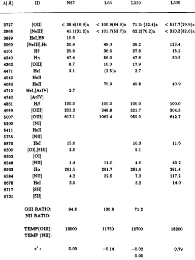
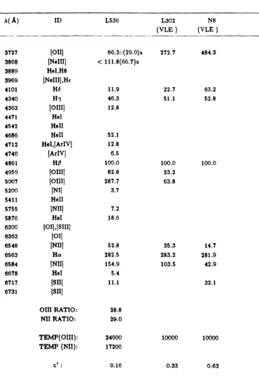
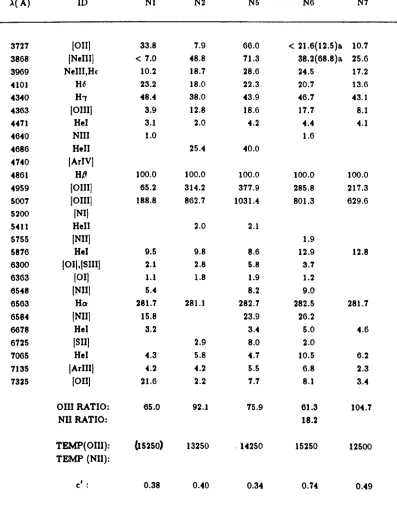
2.1 Corrected relative line intensities
(a) LMC PN : medium resolution
(b) LMC PN : low resolution
(e) SMC PN : medium resolution (d) SMC PN : low resolution . . .
2.2 Estimated errors in line intensity measurements due to uncertainty in the continuum level caused by noise 2.3 Comparison of dereddened [011]3727
A
and [NelII]3868A
line intensities with Aller (1983) and Barlow (1986)
(a) LMC PN : medium and low resolution
(b) SMC PN : medium and low resolution
2.4 Comparison of IDS relative intensities with other sources
Chapter 3
3.1 References for atomic data
3.2 [011] electron densities, from Barlow (1986) 3.3 Comparison of electron temperatures . . .
3.4 Comparison of abundances derived from medium and low resolution spectra
41
41 48 51
54
· . . . 37
· . . . 57
57 58
59
65 67 85
(b) Ionic abundances (other elements)
(c) Elemental abundances
3.6 Abundances for SMC PN
(a) Helium ionic abundances
(b) Ionic abundances (other elements)
(c) Elemental abundances . . . . .
3.7 LMC, SMC, and Galactic elemental abundances of PN and HII regions .
(a) Mean abundances
(b) Differences in mean abundances of PN and HII regions
3.8 Abundances of 'Type I' PN 3.9 Abundances of 'low oxygen' PN
Chapter 4
4.1 Absolute and IDS log F(H.B)
91 93
95
95
96
97
72
72 73
74 75
107
(a) LMC PN : medium resolution (Feb 5/6) 107
(b) LMC PN : medium resolution (Feb 6/7 and Feb 7/8) 108 (c) LMC PN : low resolution . . . 109
(d) SMC PN : medium resolution (Feb 6/7 and 7/8), and low resolution 111
4.2 Adopted values of log F(H.B), c(H.B), and log I(H.B) 113
(a) LMC PN 113
(b) SMC PN . 114
Chapter 5
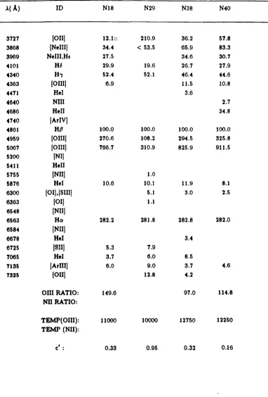
5.1 Emission line intensities for LMC N25
5.2 Ionic and elemental abundances for LMC N25
5.3 Ionic and elemental helium abundances for LMC N25
5.4 Central star parameters for LMC N25 . . . .
Chapter 6
6.1 Wolf-Rayet WC spectral classification (Torres et al., 1986) 6.2 Wolf-Rayet WC spectral classification (Torres, 1985)
6.3 Wolf-Rayet WC spectral classification for MC PN . .
135
140 141 144
162 163
Chapter 2
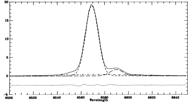
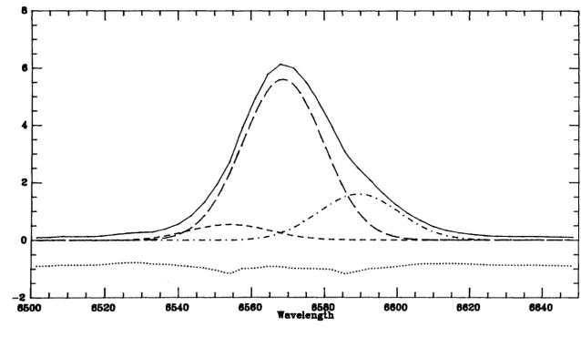
2.1 Examples of multicomponent gaussian fits for medium resolution spectra
(a) H,),[OIIIj4363A blend
(b) Ha,[NIIj6548,6584 A blend
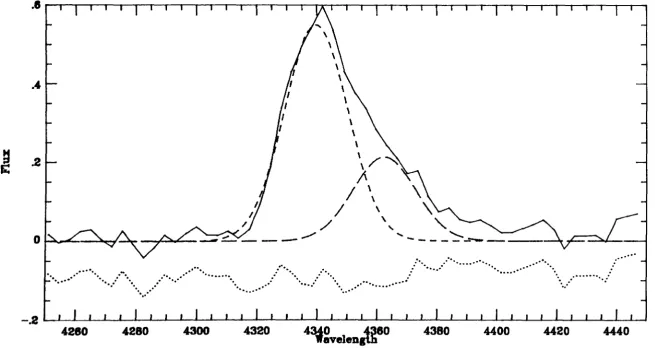
2.2 Examples of multicomponent gaussian fits for low resolution spectra . .
(a) H,},,[OIIIj4363A blend
(b) Ha,[NIIj6548,6584 A blend
2.3 Atmospheric refraction curves
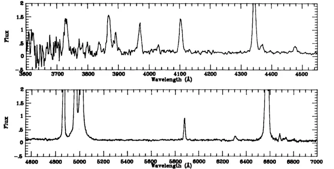
2.4 Example IDS spectra (for signal to noise comparison)
(8) LMC N123 : medium resolution
(b) LMC N212 : medium resolution
(c) LMC N208 : medium resolution
Chapter 3
3.1 Energy level diagram for the lowest terms of 0++ and N+
3.2 Energy level diagram for the ground configuration of 0+ 3.3 Elemental abundance variations for LMC PN
(8) log N/H tiS. He/H.
30
30 31
32
32 33
34 38
38 39 40
3.4 Elemental abundance variations for SMC PN
(a) log N/H VB. He/H
(b) log O/H VB. He/H
(c) log N/O VB. He/H
(d) log N/H VB. log O/H
Chapter 4
4.1 Comparison of the energy spectrum of model atmospheres and
Black Bodies . . . .
(a) Kurucz 40000 K, log g 4.0, and Black Body 40000 K
(b) Mihalas 40000 K, log g 4.0, and Black Body 40000 K .
4.2 Log G(T~) variations with effective temperature
(a) Mihalas model atmospheres
(b) Kurucz model atmospheres .
4.3 Comparison of central star parameters with theoretical
evolutionary tracks of NPN (Schonberner, 1979,1983)
4.4 Decomposition of the optical and ultraviolet spectra
of LMC N201
Chapter 5
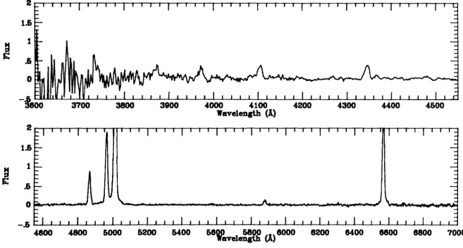
5.1 IPCS narrow slit spectrum of LMC N25
5.2 IPCS wide slit spectrun of LMC N25 .
5.3 IDS medium resolution spectrum of LMC N25
81
81
82
83
84
101
101
102
104
104
105
124
130
136
137
6.1 IDS medium resolution spectra of LMC VLE's
(a) N16 (b) N47
(c) N99
(d) NI0l
6.2 IDS medium resolution spectra of SMC VLE's
(a) N8
(b) L302
6.3 Wolf-Rayet spectral features of LMC NllO
(8) 4400
A
to 4800A :
(b) 5500A
to 6000A :
medium resol u tion154
154 155
156
157
158
158
159
166
6.4 Wolf-Rayet spectral features of LMC N133 . . . 167
(8) 4400
A
to 4800A :
(b) 5500A
to 6000A :
medium resolution6.5 Wolf-Rayet spectral features of LMC N203 . . . 168
(8) 4400
A
to 4800A :
(b) 5500A
to 6000A :
medium resolution6.6 Wolf-Rayet spectral features of SMC N6 . . . 169
(8) 4400 A to 4800 A : (b) 5500 A to 6000 A : low resolution
6. T Wolf-Rayet spectral features of SMC N6 . . . 170
(8)
4400 A to 4800 A : (b) 5500 A to 6000 A : medium resolution6.8 Wolf-Rayet spectral features of SMC L302 . . . 171
CHAPTER 1
Introduction
In this introductory chapter earlier theoretical and observational work will be
re-viewed to provide a background for this study, and the aims of the study will be defined.
In a survey of the size reported here (74 objects in two local galaxies) the analysis
touches upon many different aspects of interest in current astrophysics research. To
restrict the length of this introductory discussion, therefore, only those topics directly
related to the main analysis will be included; that is, the elemental abundances and
central star parameters of Magellanic Cloud planetary nebulae (MC PN).
The aims of this study are defined in the final section of this chapter, § 1.4.
1.1
Distance, reddening, and gas phase elemental abundances
of the Magellanic Clouds.
This section briefly reviews the recent determinations of distances to the Large and
Small Magellanic Clouds (LMC and SMC), and outlines a method for the determination
of interstellar extinction for individual objects in each galaxy, §1.1.1 and §1.1.2. This is
to be satellites of our own galaxy. Both the LMC and SMC are relatively nearby (within
60 kpc), and for this reason present the rare opportunity of observing individual objects
within a galactic system at a different evolutionary phase to our own.
The main methods used for the determination of the distance to these nearby
galax-ies are the studgalax-ies of the periods of RR Lyrae and Cepheid variables, where the
period-luminosity relationship is used to derive absolute brightnesses, and thus distances to
these objects. Observations of RR Lyrae stars have recently been used to determine the
distance to the LMC by Reid and Strugnell (1986), who by comparison with distances
determined from other methods {Cepheid stars, Main Sequence fitting, and OB stars}
suggested a 'best bet' distance of 47.5
±
2 kpc for the LMC, and, following a similar comparison, 57.5± 3 kpc for the SMC. The small errors on both of these distances,
and the small additional error in assuming all objects in a galaxy to be at the same
distance, is in contrast to the highly uncertain distance scales used for Galactic PN. One
of the main advantages of observing PN in the Magellanic Clouds is that with accurate
distances, reasonably accurate estimates of the luminosties of PN central stars (NPN)
can be made. Coupled with a derived stellar temperature this allows the NPN to be
directly compared to theoretical evolutionary tracks in the log L, log T '-II plane of the
HR diagram (§1.2).
A recent complication to this situation was reported by Mathewson
et
at.
(1986)who from a study of Cepheid variable stars in the SMC, determined a depth to the SMC
of 32 kpc, with a range of distances from 43 kpc to 75 kpc, although the maximum
concentration of objects was at 59 kpc in agreement with the Reid and Strugnell (1986)
result. The uncertainty of assuming a single distance for all objects in the SMC is
therefore ±27%, and could have a significant effect on some objects although the mean
value of parameters determined from a single distance should not be greatly affected.
1.1.2
Interstellar extinction to the LMC and SMC.
ac-Chapter 1
Coulson, 1985), values that do not vary by a great deal over the face of the two
galax-ies. The situation for the Galaxy is rather different and Galactic objects can have very
large extinction along their line of sight, with individual values varying dramatically
throughout the Galaxy (Burstein and Heiles, 1982). For PN, however, the optical
spec-tra provide a sspec-traightforward method for determining this reddening, by correcting the
flux ratio of the hydrogen Balmer series to the theoretical values (Brocklehurst, 1971)
using a reddening law derived for galaxy in question. For the spectra analysed in this
study, though, the large atmospheric dispersion affect (§2.3) meant that the
individ-ual reddening of the objects observed could not be derived by this method. Therefore,
rather than adopt a single mean reddening for each galaxy, the reddening for each
in-dividual object was determined from the column density of neutral hydrogen, N(H
I),
and relationships derived between it and the interstellar extinction as measured by
E(B - V).
To determine the extinction to individual objects, then, each object was assumed
to have a known amount of Galactic foreground reddening, plus a reddening component
local to the appropriate cloud. The Galactic foreground component was estimated from
the maps of Burstein and Heiles (1982), which give contours of E(B - V) in steps of
0.03, and only varied slightly from one object position to another. To determine the
LMC or SMC contribution the following gas to dust ratios, determined from Lyman-a
profile fitting (Bohlin, 1975), were adopted:
N (H I) 22 ( 2 1)
E{ B _ V) = 2 x 10 em - mag - ,
for the LMC (Koornneef, 1982); and
N(H I) 22 ( 2 1
E(B _ V) = 8.7 x 10 em- mag- ),
for the SMC (Fitzpatrick, 1985). By determing the column density of neutral hydrogen
neutral hydrogen column density, will not be accounted for in this analysis, and that
some objects will have an actual reddening significantly different to that adopted.
It is of interest to note here that the derived gas to dust ratios for the LMC and
SMC are greater than that of the Galaxy (4.8 x 1021cm-2mag-1
, Bohlin et ai., 1978)
by factors of .. an 18 respectively, and that both appear depleted in dust with respect
to that in the Galaxy. The dust that is present in the LMC and SMe also appears to
differ in extinction properties to the Galaxy, with the distinctive bump at 2200 A seen
in the extinction curve of our own galaxy barely present in that of the LMe, and not
discern able in the extinction curve of the SMe (Nandy, 1984; Howarth, 1983). These
differences in extinction curves are marked in the ultraviolet region, with the optical
part of all three curves being remarkably similar. From the point of view of correcting
an optical spectrum the reddening curves are essentially identical.
In terms of element abundance, Nandy (1984), using the grain size distribution of
Mathis tt al. (1977), was able to fit the extinction curve of the LMe with a graphite contribution 35% of that used in fitting the Galactic 2200
A
feature, and the SMe with a nil contribution from graphite. This result implies a depletion of graphite (assumingit to be responsible for the 2200 A feature) from the Galaxy, to the LMe, and finally to
the SMe. Similarly, the result can be seen as a depletion of carbon through the three
galaxies, a suggestion that is further substantiated by an observed decrease in gas phase
carbon (as measured by H II regions) across the three galaxies (Dufour et al., 1982).
1.1.3
Gas phase elemental abundances in the Magellanic Clouds.
The trend of decreasing carbon abundance in H II regions from the Galaxy, to the
LMe, and the SMe, is a recent result which reflects the general depletion of other
elements through the three galaxies as reported in earlier studies of H II regions. A
review of this work since 1974 is given by Dufour (1984) and brings together the work
Chapter 1
significantly depleted with respect to the Galaxy in these elements (a good summary of
these results is given in Table 3 of Dufour (1984)).
The importance of the H II region abundances is that they provide the gas phase
elemental abundance from which, presumably, the PN were formed, and direct
com-parison of H II region elemental abundances with PN elemental abundances provides a
measure of the enhancement (or otherwise) of each element during the lifetime of the
PN progenitor. A comparison of this type is made for MC PN and MC H II regions
in §3.4 using the elemental abundances derived in this study and the "recommended
abundances" of Dufour (1984).
1.2
Elemental abundances and evolutionary theory for Galactic
PN.
In this section the review of Galactic PN will be restricted to a discussion of the
typical abundances ofthese objects, §1.2.1, and a short summary of the elemental
abun-dances of Halo PN, §1.2.2. Subsection 1.2.3 presents 8 summary of the classification of
'Type I' PN, and of the 'dredge-up' processes thought to be responsible for the He and
N enhancement in these objects. Finally, in §1.2.4, a short discussion of the problems
involved in comparing the central star luminosities of Galactic PN with those predicted
by PN evolutionary theory, is presented.
1.2.1
Elemental abundances of Galactic PN.
Decades of observations of Galactic PN have provided a mass of data which provide
a consistent and thorough evaluation of elemental abundances in these objects. A recent
survey of 41 Galactic PN by Aller and Czyzak (1983 a) provides a good example of the
can be used as 'typical values' (by far the vast majority of PN), second, the elemental
abundances of 'low-Z' or 'Halo' PN, and last the elemental abundances of 'Type I' PN (those enriched in He and N).
The 'typical' PN give a reasonably consistent picture of elemental abundance, with
nitrogen, oxygen, neon, sulphur, chlorine, and argon having mean abundances by
num-ber of 8.26,8.64,8.03,7.00,5.22, and 6.43 respectively (12
+
log X/Hi Aller and Czyzak, 1983 a). The helium abundance of these Galactic PN, excluding objects where thereis a large fraction of neutral helium, provides a remarkably consistent value of 0.110.
Compared to Galactic H II regions (see Table 3.7{a)) He, N, and C are enhanced, whilst
the other elements remain approximately unchanged.
1.2.2
Elemental abundances of 'Halo' PN.
A small number of PN observed in the Halo of the Galaxy display remarkably low
elemental abundances compared to typical PN and Solar abundances. Table 3.9 presents
the abundances offour ofthese 'Halo' PN (K648, H4-1, BB-l, and DOOM-I) taken from
the studies of Torres-Peimbert et al. (1981) and Barker (1980,1983). They are depleted, with respect to typical Galactic PN, in N, 0, Ne, S, and Ar by approximate factors of 4, 7, 9, 100, and 100 respectively, although important variations do occur from object
to object (Clegg et al., 1986).
1.2.3
Galactic 'Type
I'
PN.
A third distinct group of Galactic PN (in terms of elemental abundances) are those
which display enhancements of He and N (or N/O) compared to typical PN abundances,
the 'Type I' class of PN defined by Peimbert and co-workers (see Peimbert and
Torres-Peimbert, 1983) from the following criteria;
He/H ~ 0.125 and log N/O ~ -0.3.
Chapter 1
The three 'dredge-up' processes, thought to occur when the base of the convective
envelope extends inwards (in mass) to regions rich in material processed by stellar
nucleosynthesis, are fully reviewed by Iben and Renzini (1983), and only a summary of
the changes to the surface abundances will be given here.
(1) On becoming Red Giants for the first time (following exhaustion of central
hydrogen), the star experiences the first dredge up phase, which alters the surface
ele-mental abundances of nitrogen (roughly doubled), helium (slight increase), and carbon
(reduced by 30% ), with oxygen staying roughly the same.
(2) Following the exhaustion of central helium, and the formation of an
electron-degenerate core, the most massive AGB stars undergo a second dredge-up where up
to 1 M0 of He rich material can be added to the convective envelope. This dredge up of material from a hydrogen depleted zone further enriches the surface nitrogen and
helium abundances, and depletes the surface carbon abundance. The detailed changes
vary with initial mass and metalicity, and are given in Becker and Iben (1979).
(3) The third 'dredge-up' phase occurs during the final stages of AGB evolution and
is a combination of several mixing episodes. In each case, following a helium shell flash
(thermal pulse), significant amounts of He and C are added to the convective envelope,
giving a further increase in helium surface abundances, and an increase in the surface
carbon abundances following the decrease of the earlier to 'dredge-up' phases.
The correlation between increasing helium abundance and increasing nitrogen
abun-dance for 'Type I' PN is thought to be a consequence of the second 'dredge-up', and
the final dredge-up of carbon provides an explanation for the grouping of M, S, and C
stars up the AGB (Iben and Renzini, 1983; Wood et al., 1983). The difficulties with
the Galactic PN distance scale, however, does not allow accurate determination of NPN
luminosities and masses, which severely hinders comparison with the 'dredge-up' theory.
theory (which follows the star from Red Giant to White Dwarf), in the log L, log T,,,
plane of the HR diagram.
The standard theoretical work of PN central star evolution is that of Schonberner
(1979,1981,1983), following earlier work by Paczynski (1971,1975). The Schonberner
models take various intermediate mass AG B stars that are in the thermal pulse phase
of evolution, and evolve them into NPN during an interpulse period. Steady mass
loss is included in the models but does not explain the total removal of the hydrogen
rich envelope (Schonberner, 1979). The timing of the onset of the PN phase in the
interpulse period produces models that cross the HR diagram and move down to the
White Dwarf region in times comparable with the derived age of PN (30000 - 40000
yrs.; Schonberner, 1983). Some models of lower core mass have been calculated for
higher mass loss rates, and for a final thermal pulse after PN ejection (Schonberner,
1983). The main conclusions from this work are that only 20% of post-AGB stars will
undergo a thermal pulse, and that the lower limit for the luminosity and mass of the
central stars of PN are 2500 L0 and 0.55 M0 respectively.
The NPN evolutionary tracks were calculated for two pairs of core masses, 0.64 M0
and 0.60 M0 (Schonberner, 1979) and 0.565 M0 and 0.546 M0 (Schonberner, 1983).
The main features of the tracks are the near horizontal (constant luminosity) evolution
of the central star across the HR diagram from the tip of the AG B, followed by a
sudden drop in luminosity and slow decrease in temperature towards the White Dwarf
region (occuring at "" 100000 K). The luminosity of the 'horizontal' part of each track
is directly associated with the core mass and interpolation between the tracks to derive
core masses between the tracks can be done with reasonable accuracy, as shown by the
extrapolated low core mass tracks of Schonberner (1981) and the calculated low core
mass tracks of Schonberner (1983) In this study they are used for comparison with
derived NPN luminosity and temperature in an HR diagram (Fig. 4.3).
For Galactic PN Pottasch (1983) has shown that some measure of agreement exists
luminosi-Chapter 1
Peimbert and Torres-Peimbert (1983), NGC 6751, NGC 6629, and NGC 7008, a further
'Type I' PN lies just above the 0.60 M0 track, NGC 6537. These positions are odd
as the central stars of 'Type I' PN should evolve from the higher mass end of the PN progenitor mass range, and form NPN with core masses at the higher end of the range,
i.t ... 0.8 M0 (Iben and Renzini, 1983). Assuming the 'Type I' PN to be wrongly placed by ... 0.2 M0 in Fig. 6 of Pottasch (1983), it is easy to visualise moving the
entire sample of 50 PN up in luminosity by a factor of 3 or so, to fall around the 0.6
M0 track with a few PN near the 0.8 M0 track (including the 'Type I' PN mentioned
above). It seems possible, therefore, that the distances adopted by Pottasch for these
PN are still not correct, a suggestion that is further supported by the fact that many
of the NPN have derived luminosities below the lower limit of 2500 L0 suggested by
Schonberner (1983). The importance of studying MC PN, where accurate distances are
available, is evident for comparisons of this type.
1.3
Previous studies of MC PN.
In this section previous observations of Magellanic Cloud PN are reviewed; §1.3.1
summarises the early surveys that identified MC PN, whilst §1.3.2 reviews the studies
whose aim was to derive MC PN elemental abundances. The final subsection, §1.3.3,
summarises the observations of MC PN central stars.
1.3.1
Early surveys of MC PN.
Early surveys of MC PN concentrated on the identification of these objects through
their emission line spectra and low stellar continuum level in the optical. Surveys
two galaxies. The most reliable listing of MC PN to date is given by Sanduleak et al. (1978), with additional LMC PN from Sanduleak (1984).
1.3.2
Elemental abundance studies of
Me
PN.
Detailed chemical abundance studies of MC PN were not possible until 1976 when
Osmer (using a photoelectric scanner) observed 3 LMC PN (WS 7, WS 8, and WS 40;
or N97, N24, and LMI-61 in the nomenclature of this study) and 3 SMC PN (N2, N54,
and N67), although an objective prism study by Sanduleak et al. (1972) did indicate a general nitrogen deficiency in the LMC and SMC PN.
The study by Osmer (1976) reported evidence for an overabundance of helium by
_ 40% and an underabundance of oxygen by a factor of 10 in the SMC and 3 in the
LMC. The NjO ratio was found to be similar to that of Galactic PN.
Dufour and Killen (1977) (using photographic image-tube techniques) also observed
SMC N67 and LMC N97, along with LMC NI53 and 3 H II regions. They found SMC
N67 to have a high helium abundance, in agreement with Osmer (1976), but that the
two LMC PN had normal helium abundances with respect to Galactic PN. Additionally,
the oxygen abundances displayed the same trend as those reported by Osmer (1976),
and the NjO ratio was found to be significantly larger than that measured in MC H II
regions.
More recently, Aller and his co-workers have observed 7 SMC PN (N2, N5, N43,
N54, N70, and N87; Aller et al., 1981), and 8 LMC PN (NI84, N97, N24, NI02, N153, N178, N201, and LMI-61; Aller. 1983; Maran et al., 1982; Aller and Czyzak, 1983 b).
For the LMC PN, Aller (1983) concluded that the helium abundance was greater
than in the LMC H II regions and comparable with the Galactic PN abundance, except
that N97, N201, and N178 were all helium rich. Two LMC PN were found to be nitrogen
rich, N24 and N201, but the other objects displayed nitrogen abundances greater than
LMC H II regions and less than Galactic PN. Oxygen was found to be strongly depleted
Chapter 1
PN. Whilst the oxygen abundance was comparable with SMC H II regions but less than
that of Galactic PN.
More recent work by this group (Maran et al., 1982; Stecher et al., 1982) reports the ultraviolet spectra of 3 MC PN, presenting nebular carbon abundances, stellar
luminosities, and core masses. This small, but important, study was extended to 12 MC
PN (6 LMC and 6 SMC) by Gull et al. (1986) who revised the central star luminosities reported earlier by Stecher et al. (1982) downwards by factors of 6-12. The conclusions of this series of ultraviolet observations, summarised by Gull et al. (1986), are that carbon and nitrogen are enhanced by factors of 10 in the SMC and 4 in the LMC
compared to H II regions, and that elements other than carbon are deficient in MC PN
compared to Galactic PN.
From the results of the Gull et al. (1986) survey, the mean carbon abundance of LMC PN, excluding possible 'Type I' objects (N97, NI02, and N201), is 8.56 (12
+
log X/H). For SMC PN, excluding N67, the mean carbon abundance is 8.65. In each galaxy,excluding possible 'Type I' objects, the PN have C/O> 1. The 'Type I' candidate MC
PN all showed lower carbon abundances (7.34,7.49,7.27, and 6.27 for LMC N97, LMC
NI02, LMC N201, and SMC N67 respectively), possibly showing a strong depletion of
carbon during the second 'dredge-up' phase.
Compared to the mean carbon abundance of Galactic PN (Aller and Keyes, 1986)
and LMC and SMC H II regions {8.71, 7.9 and 7.16 respectively (Dufour et al., 1982)), the 'normal' He/N abundance MC PN reflect the same pattern for carbon abundance
u the other elements, falling between Galactic PN and MC PN H II region values.
The difference between the Galactic PN and MC PN abundances is not very large,
however, whilst the differences between PN and H II region carbon abundances in the
Galaxy, the LMC and the SMC are 0.25 dex, 0.66 dex, and 1.49 dex, respectively.
This indicates a strong correlation between increasing carbon abundance enhancement
for such determinations, and any conclusions drawn should be weighed against these uncertainties.
1.3.3
Central star studies of MC PN.
Despite the importance of observing MC PN central stars, for comparison with theoretical models of NPN evolution, very little work has previously been carried out in this area, due to the difficulty of detecting the stellar continuum at the distance of the Magellanic Clouds with present day instruments. At the temperatures of the majority of NPN the stellar continuum is brightest in the ultraviolet, but to detect it requires long exposures (- 4 hours) with JUE. Observations of the stellar continuum in the optical are feasible (see Chapter 4 of this study) but only sample those PN with lower stellar temperatures (25000 - 50000 K).
Only one ultraviolet survey of MC PN central stars has been reported: Gull et ai. (1986, and references therein). This has provided an indication of the possibilities in this field, although the recent revision by this group of their derived stellar luminosities also reflects the problems involved and the care needed in the analysis. The final stellar luminosities and masses derived for the central stars in the survey of Gull et til. (1986) fall within the range 3500 - 11200 L0 and 0.58 - 0.71 M0 respectively, in good agreement with the NPN evolutionary tracks of Schon berner (1979,1983), although no direct comparison was made by the authors.
1.4
The main aims of this study.
Chapter 1
(2) The determination of mean He, N, 0, Ne, and Ar abundances for LMC and
SMC PN from a large sample of objects (but excluding anomalous abundance PN),
for direct comparison with mean elemental abundances of Galactic PN and Magellanic
Cloud H II regions.
(3) The determination of elemental abundances for MC PN defined as 'Type 1', for
comparison with Galactic 'Type I' PN and with theoretical predictions.
(4) The derivation, where possible, of stellar temperatures and luminosities for MC
PN central stars, for direct comparison with the theoretical NPN evolutionary tracks of
Observations and Calibration
In this chapter the basic details of the observations are presented (§ 2.1), and are followed by a discussion of the technique used to deconvolve the important emission line
blends of the spectra (§2.2). The final section (§2.3) discusses atmospheric dispersion
and its correction in this data set, and includes, in Tables 2.1 (a) to (d), the corrected
relative line intensities for the 74 objects studied in this survey.
2.1
Observations
The observations were made by E. J. Wampler with the 3.9 m Anglo-Australian
Telescope (AAT) at Siding Spring Observatory during the nights of 27/28 November
1975 (low resolution data), and 4/5, 5/6,6/7, and 7/8 February 1976 (medium resolution
data), using the Boller and Chivens Spectrograph and Image Dissector Scanner (IDS)
(Robinson and Wampler, 1972), at the F /15 focus. The low resolution spectra were
obtained with a 300 line/mm grating, giving a noise-limited useful wavelength range
from 3600 A to 7400 A , at a resolution of ,.., 25 A FWHM. The medium resolution
Chapter £
of 20 arc sec. The object spectra were then summed and the sky spectra, which had
been recorded simultaneously in the alternative slots, were subtracted in order to yield
net spectra. All of the low-resolution spectra were obtained on the night of November
27/281975, when the PN were observed in essentially Right Ascension order. The same
order of observation applied on the nights of the medium-resolution observations. The
medium-resolution observations of the SMC PN N6, L239, L302, and L30S were obtained
on February 7/8, while the remaining SMC medium-resolution data were obtained on
February 5/6.
The spectra were wavelength calibrated with respect to comparison exposures of a
He-Ne arc, and were calibrated spectrophotometrically by observations of white dwarf
stars from the list of Oke (1974), using the SDRSYS reduction routine at the AAO
(Straede, 1980). The subsequent analysis of the calibrated spectra was carried out at
the VCL STARLINK node, using the DIPSO package ofroutines (Howarth and Maslen, 1984) to measure line intensities.
2.2
Deconvolution of major emission line blends.
Several groups of lines were only partially resolved in both series of spectra, most
importantly the [N
III
6548A ,
6584A
and HQ lines, and the H1 and[01111
4363A
lines, which are used either for the determination of interstellar extinction and atmosphericdispersion, or as temperature diagnostics. To deconvolve these lines into their respective
components the DIPSO routine ELF written by Dr. P. J. Storey was used. The routine provides a multi-component fit, with either gaussian or user-defined profiles, where each
component, ", is of the form;
To deconvolve the blend the routine performs a least squares fit to the observed
data by minimising the function
where
!.,l .•
is the observed flux at point Xm , the sum n is over the number of components,and the sum m is over the number of observed points.
For all blend deconvolutions gaussian profiles were adopted and the fit procedure
was carried out in wavelength space. The constraints to the fit were the theoretical line
centres (in terms of the wavelength differences from the strongest line in the blend),
and, for the (N II 6548
A
,6584A :
Ho ) blend, a relative intensity ratio of 3:1 for the nitrogen lines, from the ratio of their transition probabilities (as they both originatefrom the same excited level). The value of the FWHM was not constrained in the
procedure, except that the FWHM of similar components should be equal, but fits were
only accepted for FWHM's within,... 3
A of the FWHM of the unblended lines of the
spectrum.
The fitting was made more complicated by the presence of broad wings on the
stronger lines (those with intensity ~ 100 relative to H,8 for a typical PN), which are a
feature of the instrument itself, and whose width increased with increasing line intensity.
However, the full profile (including the broad wings) of the strongest, unblended line,
H,8, could not be satisfactorily scaled up to fit the line profiles of the NIl, Het blend, as
the strong broad component was far more prominent in the NIl, Ha: blend than in the
H,8 line It was necessary, therefore, to estimate the FWHM of this broad component
from the (unblended) H,8line, and fit both a narrow and broad component to the strong
lines within the blends. Another technique would have been to use the H,8 profile as a
standard profile and to deconvolve the blends with this rather than a gaussian shape.
The main drawback to this technique is that the width of the broad wings varied with
the line intensity, 80 that the H,8 profile would only match in shape a line of similar
(,.)
o
~5~1~'-T-~~~~-r~~~~~~~-r~'-~~~~~-r~~~~~~~-r-r'-~T-r-~~-r-r~~~
2
1.5
~
1
.5
o
t _
\~ ~
~
,
---~-
- - - -
~
~--=::-.=~---"...- ~I
~
~
....
'"
...
w
-~
15
10
5
'/ ,
I '
-/
,,...
~O r
t
- - ~... - . - . - . - . - .
- - - - ---,.,,~. - . - .
- - - -~~~:::z:-===-=-=-:"~s:2::P=-::c - ________--I
~ Q
~ ...
."
...
Co)
t.:I
·8 r I x
.4
~
.2
o~< >,</~ /><
\
\
'\
'....
""-- ""-- ""-- ""-- ""-- ""-- ""-- ""-- --..ltt
.
~
{;....
w
w
~
8"
2
;--"
/
\
'I
\
'/
\
'I
\
'/
\
'/
\_.,
/
...
\
.'.
.
"
'
/
.
...
.
,
l-:
====::::::::==:-;:;~ -~-
- - - -- . ,/
" .
.... .
--O - .... ___ . _ . _ . _ . _ . _ . -~ " .-" .... -- - - - _ _ _ _ _ _ ..::::r--_ ... ...-:.:...=-:::;:. ~ __ ==-===~=
" ... ""." ... " ... " ... . ... " ... "" ... "." ... " ... " ... "" ... " ... " ... .
~
A ~....
"
....
Chapter f
DIFFERENTIAL REFRACTION ollset relative to 5500 A
80~--~--~----~--~--~----~--~--~----~---.--~
70
60
':?
i' 50
~ w
u
Z 40
~
Cf)
o
:I: 30
~
Z
W
N 20
10
3000 A 3400';' 4000';' 5000 A eoooA 1.0 ~ - - A ( I I
t2 ~
O~--~--~--~--~~--~--~~~~~L---~--~--~ ·12 ·10 -8 ·6 ·4 ·2 0 2 4 6 8
OFFSET (ARCSEC)
Figure 2.3
Atmospheric dispersion curves: showing the offset relative to 5500
A
lor a range0/
wavelengths/rom 9000A
to 8000A
the range 5% to 15% , depending on the relative strengths of the components involved. There was more significant blending, however, in the low resolution spectra, and errors
of about 10% to 30% are estimated. It should be noted that the H1,
10
III] blending was particularly pronounced in the low resolution spectra, and the weakest [0III1
4363 A relative line intensities have the highest associated errors.about 40 degrees) the image is offset by more than 1 arc sec for wavelengths less than
- 4500 A , and less than 1 arc sec for wavelengths between 5500 A and 7000 A. For
large entrance apertures, and good 'seeing' conditions, these offsets have a negligible
effect, as the image is still fully within the aperture for all wavelengths. However, when
a narrow entrance aperture is in use, and the 'seeing' is of the order of the aperture size
(as was generally true for all spectra in this data set) any image offset will lead to a loss
of flux, and will be worse at shorter wavelengths, as an increasingly large proportion
of the image at these wavelengths falls outside of the aperture. The effect under these
conditions is not disimilar to that of interstellar extinction, in as much as the differential
offset is greater at the blueward end of the spectrum, leading to an overall reddening of
the spectrum.
The magnitude of the effect is dependent on the exact zenith distance, the entrance
aperture (i. e. slit width), and the 'seeing' at the time of the observation, and for this
data set it could only be corrected for empirically. To do this it was assumed that there
would be a reasonably linear relationship between the flux 'extinction' and wavelength
for the atmospheric dispersion and that it would follow a similar trend to the interstellar
extinction between 3500 A and 7000 A . Following a single, combined, correction for
both atmospheric dispersion and interstellar extinction, using the reddening law of
Howarth (1983), any deviations from the above assumption are corrected for empirically
by comparison between the flux intensities of PN in this data set with those in data
sets not as greatly affected by atmospheric dispersion.
All spectra were, therefore, first corrected to the theoretical Ha:Hp intensity ratio (Brocklehurst, 1971), using a galactic reddening law curve (Howarth, 1983) with a
suitable value for the logarithmic constant (c' in Tables 2.1(a) to 2.1(d». The galactic
law was used for the total dereddening rather than seperate curves for the LMC, SMC,
and our own galaxy, as the various extinction laws of the three galaxies longward 3500
A
are almost identical (Howarth, 1983; Nandy, 1984), and any of them would serve as an
Chapter
t
Following this correction, the effects of atmospheric dispersion were, as expected,
most pronounced at the blue end of the spectra and further corrections were found to
be necessary to the fluxes of the lines shortwards of 4400
A .
In order to estimate the magnitude of the corrections needed, two types of comparison were made. First thecorrected relative intensities of [011]3727
A
and [Ne III] 3868A ,
were compared with the dereddened relative intensities for these lines from Aller et 0.1. (1981), Aller (1983),and Barlow (1986), for the nebulae in common. The relevant line fluxes are listed in
Tables 2.3(a) (LMC PN), and 2.3(b) (SMC PN). A summary of the mean ratios of
the IDS intensities to the other intensities is presented in Table 2.4. Secondly, the
corrected H')':H~ and Hc5:H~ ratios obtained from the IDS spectra were compared to
the theoretical ratios for T~
=
10" K and Ne=
10" cm-3, 0.469 and 0.259, respectively
(Brocklehurst, 1971). A comparison between the observed mean ratios and theoretical
ratios is also included in Table 2.4.
Inspection of the various ratios in Table 2.4, for the low resolution spectra of both
the SMC and LMC PN, indicates that the corrections needed for the [0
III,
[Ne III], Hc5, H')' fluxes are similar. The weighted mean of all 93 low resolution ratios (IDS divided byother) is 0.89. All low resolution line fluxes between 3700
A
and 4400A
have therefore been multiplied by a factor of 1/0.89 (= 1.12). The corrected low resolution line fluxeslisted in Tables 2.1(b) and 2.1(d) are thus the result of the dereddening of all fluxes by
c', followed by multiplication by a factor of 1.12 for those lines with ~ < 4400
A .
In the case of the medium resolution spectra, the dereddened to intrinsic Balmer
line ratios in Table 2.4 indicate that a correction factor of 1/0.89 (= 1.12) is again
appropriate for H6 and H,)" for both the SMC and LMC PN. However, in the case
of the [0
II]
and [Ne III] lines, the ratio of the medium resolution IDS to others is significantly lower than 0.89. This additional reduction in flux at short wavelengths wasattributed not to atmospheric dispersion, but to the fact that these lines fall close to
Table 2.2 Estimated errors in line intensity measurements due to uncertainty in the continuum level caused by noise.
ReJl\tive
IntensIty Wavelength Rl\nge (Angstroms)
(HP=loo) < 3900 3900-4200 4200-6000 6000-7000
3-5 > 50 % > 50 % 40 % 30 %
5-15
..
30-40 % 20-30 % 20 %15-35
..
25 % 10-15 % 10 %> 35 > 30 % 10 % 10 % 10 %
the result of the dereddening of all fluxes by c', followed by multiplication of the above
correction factors.
The final corrected relative line intensities (on a scale where HP = 100) are presented separately for the medium and low resolution spectra of the LMC PN (Tables 2.1(a)
and 2.1(b), respectively), and the SMC PN (Tables 2.1(c) and 2.1(d), respectively). The
estimated errors of measurement of the relative line intensities are listed in Table 2.2,
and are a function of (a) the wavelength, (b) the line intensity (relative to HP), and
(c) the overall strength of the signal. These effects will combine to produce a specific
signal-ta-noise ratio for an individual line within a spectrum, and the estimated errors
are the uncertainty due to the noise over the various wavelength regions. Figs. 2.4 (a),
(b), and (c) show example spectra from the dataset to illustrate the signal-ta-noise ratio
variations over the wavelength range analysed. Spectra with a weak overall signal have
higher auociated uncertainties, and these spectra have been labelled by an asterisk next
to the object name in Tables 2.1(a) to 2.1(d). For these spectra, and for other spectra
with non-detections of the important [0 IIJ3727
A
and [Ne IIIJ3868A
lines, upper limitsto the fluxes in these lines were measured. For some nebulae for which only upper limits
""
011
~
~
2
i I i1.&
1
.&
o
3700
3800 39004000
·4100
42004300
Wavelenllh
(1)
4400
2
i • i i . 'I • ii'1.&
1
.&
4500
~
A ~....
'"
..
~
~
co
~
1.6
1
.6
0
-feoo
3700
38003900
4000
4100
4200
4300
4400
Wavelen,th
(.1)
2
r-.
' • ' , ',I"
.
' , ,.
' ,.
' ,...
•
• • • •
'n •1.6
t:-
1111II
11:...
II II
II
.6
4600
• • • '""1
-:l
~
~'1:3
....
."
...
....
o~
~
2
i Ii iIi i iI1.6
1
.6
o
3700 3800 3800
4000
4100
42004300
4400Waveltm.1lh
(.1)
2 ,
_,
...
i i iIi1.6
1
4600
~
~
~
....
'"
..
Table 2.1{a) Corrected relative line intensities for LMC PN : medium resolution
ID Nl N25 N42 N52 N60 N66
3727 lOll] < 28.9 58.9 < 101.0 < 30.9 < 32.1 < 86.2(60.6)a 3868 INeIll] < 28.1 < 19.2 < 119.1 66.7 45.7 103.1(112.2)a
3889 Hel,H8 33.3:: 22.6 22.8
3969 INeIII],Hf 18.0 < 64.8 42.5 19.2 15.4 4101 Hc5 27.2 31.5 30.4 20.4 24.8 27.5 4340 H, 44.1 48.7 39.8 52.5 47.8 49.3 4363 10Ill] 8.9 < 9.7 30.6 13.2 6.0 18.7
4471 Hel 4.8 4.5
4542 Hell
4686 Hell 23.8 60.2
4712 Hel,IArIV] 5.8 15.0
4740 IArIV] 5.3 8.7
4861 HP 100.0 100.0 100.0 100.0 100.0 100.0 4959 10Ill] 128.6 17.4 448.3 418.0 222.4 319.0 5007 10III] 398.0 47.7 1403.8 1238.3 647.2 973.8 6200 INII
5411 Hell 6.8
5755 INII] 3.2 2.6
5876 Hel 13.S 4.9 IS.8 11.1 13.4 7.7 6300 101] ,ISm] 1.5 2.5 11.9 2.8 10.0
6363 1011 0.9 3.5
6548 INII] 1.6 17.1 21.9 0.6 4.3 40.0 6563 HQ 282.3 282.8 282.6 282.7 282.4 282.2 6584 INII] 4.6 49.8 63.8 1.6 12.7 117.0
6678 Hel 3.8 4.4 4.3 3.4
6717 ISII] 5.8
6731 ISII] 6.9 1.8 8.0
OIll RATIO: 59.1 6.7 60.6 125.2 145.7 69.0
NIl RATIO: 21.1 59.7
TEMP(OIII): (16000) 15750 11750 11250 15000
TEMP (NIl): (21000) 11000
Chapter I
Table 2.1(a). -continutd
ID N77F N78 NI01 NI02 NI04A NllO
3727 lOll] 279.4 28.6 53.5 55.8 < 206.2 72.7 3868 INelll] 87.3 38.2 29.2 99.3 100.6 83.9
3889 Hel,H8 28.5
3969 INelll],Hf 26.1 22.2 30.5 36.2:: 50.0 4101 H6 18.9 25.7 23.6 22.7 11.5 25.2 4340 H"Y 45.4 45.8 51.5 47.6 52.1 42.7
4363 10111] 3l.4 1.6 45.7 25.1 9.8
4471 HeI 7.2 5.2 4.6
4542 Hell
4686 Hell 68.1 75.3 39.1
4712 Hel,IArIV] 12.3
4740 IArIV] 17.5
4861 HP 100.0 100.0 100.0 100.0 100.0 100.0 4959 101II] 453.5 186.5 380.0 525.0 429.9 5007 IOIII] 1382.8 549.1 2.3 1l24.8 1545.9 1l98.3
5200 INI] 10.5 12.7
SUI Hell 9.5 5.7
5755 INII] 14.4 2.9 9.0
5876 HeI 6.6 14.8 1.2 U.8 9.9 15.2
6300 101]tISIII] 30.6 2.5 3.2 26.8 11.9 13.7
6363 101] 1.8 3.7
6548 INII] 156.3 6.5 29.7 117.5 28.7 lU 6563 Ho 283.4 281.2 282.3 282.8 283.0 282.8 6584 INII] 460.9 18.9 87.0 342.8 83.1 41.2
6678 Hel 4.5 5.4
6717 ISII] 14.4 2.8 6.1
6731 ISII] 30.4 12.5 4.5
0111 RATIO: 68.4 456.1 32.9 82.6 166.0 NIl RATIO: 42.8 40.4 5l.4
TEMP(OIII): 16000 (10000) 23250 13750 10500 TEMP (NIl): 13000 13500 12000 (6250)
c' : -0.27 0.80 0.40 0.67 1.18 0.26
Table 2.1{a). -continued
ID N122 N123 N124 N125 N133 N141
3727 lOll] 52.6 37.5 34.8 38.5:: < 25.4(6.6)a 22.0 3868 INelII] 125.8 38.5 67.0 40.3:: 51.8::(37.8)a 41.6
3889 Hel,H8 22.8 15.5 17.0 10.6
3969 INelll] ,HE 50.0 24.5 36.7 22.8:: 53.2 28.1 4101 HIS 26.4 25.2 18.1 21.5 26.2 18.9 4340 H1 45.7 44.5 46.4 48.2 47.6 37.4 4363 101II] 19.0 6.1 21.8 11.3 11.2 8.0
4471 Hel 5.1 4.6 3.6 4.3 4.4 4.4
4542 Hell 2.4
4686 Hell 42.0 23.1
4712 Hel,IArIV] 6.3 0.9 4.4
4740 IArIV] 9.3 3.0
48GI Ht3 100.0 100.0 100.0 100.0 100.0 100.0 4959 101II] 367.9 229.1 521.6 341.9 251.1 344.7 5007 101II] 1066.0 G84.6 1512.6 1004.9 701.2 97G.l 5200 INI] 1.9
5411 Hell 3.2 1.5
5755 INII] 8.3
5876 Hel 15.3 13.3 10.6 14.8 13.2 13.4 6300 101] ,ISIII] 13.0 3.7 5.2 2.4 4.3 2.6
6363 101] 3.6 1.0 0.8
6548 INII] 85.2 7.8 7.0 4.8 1.8 6.2 6563 Ha 282.0 282.1 282.9 281.7 282.9 282.6 6584 INII] 250.6 22.9 20.5 14.0 5.1 18.1
6678 Hel 3.2 3.6 5.2 2.8 3.6
6717 IS II]
6731 ISII] 13.1 3.1 5.3 3.8 3.2
OIII RATIO: 75.3 148.6 93.3 119.2 85.1 164.9 NIl RATIO: 40.7
TEMP(OIIl): 14400 11000 13000 12000 13250 10750 TEMP (NIl): 13800
Chapter t
Table 2.1(a). -continued
ID NISI NI53 N170 Nl78 N181 N182
3727 lOll] < 38.3 55.6 67.5 59.5 373.2 34.3 3868 INelIl] 73.0 99.1 94.2 84.6 92.8 50.5
3889 Hel,H8 29.5 34.0 20.7 11.8
3969 INeIIl],H( 47.3 35.1 33.2 42.1 35.3
4101 H6 22.9 31.1 20.2 26.8 24.0
4340 H'Y 43.2 43.1 41.3 38.8 36.1 44.7 4363 10III] 9.9 20.6 17.1 15.5 7.2 7.1
4471 Hel 4.9 4.0 4.2 2.9 5.8 4.0
4542 Hell
4686 Hell 30.7 32.1 9.7 55.4
4712 Hel,[ArIV] 3.9 3.7 2.7 2.5
4740 IArIV] 4.5 5.9 2.9
4861 HP 100.0 100.0 100.0 100.0 100.0 100.0 4959 10III] 331.2 478.9 499.4 463.8 160.8 262.8 5007 10III] 946.2 1444.6 1481.5 1394.8 472.4 799.0
5200 INI] 31.9
5411 Hell 3.3 3.0 1.6 4.1
5755 INIl] 32.2
5876 Hel 13.9 9.7 10.3 12.1 9.8 14.4 6300 10I],[SIII] 4.3 9.2 16.4 7.0 75.6 3.7
6363 101] 2.3 4.1 2.3 23.3 0.9
6548 INII] 6.6 13.5 17.0 9.6 611.1 4.8 6563 HQ 281.3 283.3 282.1 281.1 281.8 282.3 6584 INIII 19.2 39.4 49.7 28.3 1493.0 14.2
6678 Hel 4.8 2.8 4.8 2.4 3.4
6717 ISIII 1.3 1.1
6731 ISII] 4.3 11.4 3.9 113.2
0111 RATIO: 128.6 93.2 115.8 119.6 87.6 148.8
Nil RATIO: 62.2
TEMP(OIII): 11500 13100 12000 11900 13500 11000
TEMP (NIl): 10750
c' : 0.49 0.54 0.68 0.12 0.58 -0.11
Table 2.1{a). -continued
ID NI84 NI99 N201 N203 N207 N208
3727 lOll] 56.3 78.7 35.9 < 79.7(70.8)a 82.4 76.8 3868 INeIII] 110.5 < 8.0 67.5 47.2 105.3 126.8
3889 HeI,H8 17.9 13.9
3969 INeIIlI,H£ 32.5 30.3 38.3 35.3 43.8 4101 H6 15.5 28.4 23.8 13.5 26.3 25.7 4340 H.., 38.8 37.7 45.6 39.9 44.7 47.5 4363 101II1 18.5 3.6 25.0 5.5 18.0 20.7
4471 HeI 3.7 4.3 2.9 5.2 4.0
4542 Hell
4686 Hell 45.7 25.3 43.1 25.3
4712 HeI,IArIVI 5.8 2.5 4.8
4740 IArIVI 7.4 3.5
4861 HP 100.0 100.0 100.0 100.0 100.0 100.0 4959 101II1 487.7 52.5 407.2 278.6 473.7 549.7 5007 10III] 1361.5 148.6 1144.7 800.0 1387.3 1556.6
5200 INI] 0.8 0.9
5411 Hell 6.7 3.0 4.7 1.7
5755 INIII 2.1:: 0.8 1.5 1.1
5876 HeI 10.5 6.7 12.1 15.2 10.4 12.1 6300 IOII,ISIIII 9.7 3.0 7.6 3.3 14.5 11.3
6363 1011 1.5 4.9 3.0
6548 INIII 9.1 28.0 11.4 7.7 25.8 16.2 6563 HQ 281.5 281.5 281.4 282.4 281.4 282.8 6584 INII] 26.4 82.0 33.5 22.3 75.2 47.4
6678 Hel 4.2 2.5 3.4 3.4 3.0
6717 ISIII 3.5 1.0 2.1 1.4
6731 IS III 3.9 1.7 5.5 5.3 15.3 6.3
OIII RATIO: 100.1 55.2 62.0 194.9 103.3 101.9
NIl RATIO: 51.7 59.1 67.8 57.9
TEMP(OIII): 12750 (18250) 15500 10000 12500 12750 TEMP (NIl): lt1750) 11000 10500 11250