* Supported by the Slovak Research and Development Agency under the contract No. APVV-15-0751, by the Ministry of Education, Science, Research and Sport of the Slovak Republic under the contract No. VEGA 1/0643/17 and by FVG 2017 grant
Processing of Cells’ Trajectories Data for Blood Flow
Simulation Model
*Martin Slavík +, Kristína Kovalčíková, Hynek Bachratý +, Katarína Bachratá, and Monika Smiešková
Cell-in-fluid Research Group, http://cell-in-fluid.fri.uniza.sk; Department of Software Technologies; Faculty of Management Science and Informatics, Žilina, Slovakia
Abstract. Simulations of the red blood cells (RBCs) flow as a movement of elastic objects in a fluid, are developed to optimize microfluidic devices used for a blood sample analysis for diagnostic purposes in the medicine. Tracking cell behaviour during simulation helps to improve the model and adjust its parameters. For the optimization of the microfluidic devices, it is also necessary to analyse cell trajectories as well as likelihood and frequency of their occurrence in a particular device area, especially in the parts, where they can affect circulating tumour cells capture. In this article, we propose and verify several ways of processing and analysing the typology and trajectory stability in simulations with single or with a large number of red blood cells (RBCs) in devices with different topologies containing cylindrical obstacles.
1 Introduction
Microfluidic devices with periodic obstacle arrays inside them are often used for diagnosis or even for a treatment of various diseases related to the blood. Such devices are designed for capturing, detecting and sorting rare blood cells or microorganisms. Shapes and topologies of the devices vary depending on their purpose. Many applications are in the research of circulating tumour cells (CTCs). These cells get to the blood circulation from primary tumours and can create metastasises in other parts of the human body. In [1], a device consisting of a microchannel with periodic obstacle array is described. The obstacles are covered with biologically active substance, adhesive for chosen type of cells. Obstacles without biologically active substance are used in [2]. The authors describe experiments using different angles of fluid flow inside the channel. Sometimes an array of obstacles is used, in which every row is shifted compared to the previous one [3]. This device is designed based on a diagnostics device used for extraction and enrichment of parasites from human blood. Obstacle do not have to be necessarily cylindrical, as we can see in [4], where the periodic array of obstacles with triangle cross-section is used.
Recently, computational modelling has been successfully used for investigation of rare cell behaviour in a channel with periodic obstacle arrays. One of the tools, which allows such approach is Object-in-fluid framework implemented in open source software ESPResSo [5], [6], [7]. In [6] author studies a rare cell capture rate according to the cell-fluid ratio in a channel with shifted obstacles. The cells were represented only
by spherical objects, what is a typical shape of CTC. In [7] the trajectories of single CTC were investigated in a channel with regular periodic obstacle array, with different cell densities. In this case, only CTC had a spherical shape and other cells were represented by RBCs.
The key ability of the microfluidic devices considered in this study, is their capacity to capture CTC in the blood, respectively in blood plasma. To achieve high capture efficiency, it is necessary to optimize CTC trajectories to maximize contact with obstacles. A particular problem is their very rare occurrence in blood plasma, and the small ratio of CTC compared to RBC. In the literature, it ranges from 1:5x10⁴ to 1:109. CTC will therefore be significantly affected by the RBC trajectories. In this article, we propose basic methods of investigation and statistical evaluation of the properties of RBC trajectories, mainly in terms of their stability, specifically changes in their position during their way through the obstacle array. For this purpose, we have also used Object-in-fluid framework. Due to the large computational difficulty of simulations, we examined the problem on simplified types of channels with cylindrical obstacles.
2 Simulation technical parameters
was also the direction of the periodic conditions applied which made the experiment less demanding on calculations also for models of larger channels. Cylindrical obstacles (pillars) with the radius of 5 µm were placed inside the channel. For a precise description of the channel shape, see Figure 1.
Fig. 1. Topology and proportions for channel A, channel C and orientation of coordinate axis
Each of the experiments ran for 380,000 simulation steps, which, with a time step of 0.2 µs, corresponds to the real time of the experiment of 0.0762 s. In the time, the fastest cells passed the simulated channel section many times, which means they did hundreds of micrometres in total.
All experiments were performed in the simulation software ESPResSo with usage of Object-in-fluid framework for modelling cells and LB for modelling fluid. As a model of each of the RBCs we had chosen a surface mesh with 141 nodes and the dimensions of 7.82µm × 7.82µm × 2.56µm. The elastic coefficients of the mesh were ks = 0.0044, kb = 0.0715, kal = 0.005, kag = 1, kv =1.25. The simulation mass of every cell was 0.05957 pg. The interactions among the cells were modelled by membrane collision interaction with the
parameters of mc K = 0.005, mc n = 2.0, mc cut = 0.5. The interactions between the cells and surface of the channel were ensured by soft sphere interaction with the parameters of sof t K = 0.00035, sof t n = 1.0, sof t cut = 0.5. The fluid was discretized by a three-dimensional regular lattice with the space step 1 µm. The fluid viscosity was 1.5 mPa.s and the density was 1000 kg/m3, representing blood plasma at 20 ◦C. The interaction parameter between fluid and object called friction was 0:025865531914893616. Different external volume forces were used to induce the flow in the X-direction.
3 Stability of isolated RBC trajectories
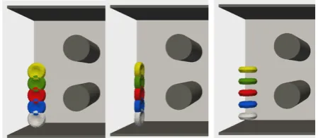
To obtain basic information about the properties of RBC trajectories in Type A and Type C channels, we first performed 15 calibration simulation experiments with a single RBC in the channel. This single RBC gradually passed through the channel from five different starting positions (with y-coordinate, i.e. the distance from channel edge, of 5, 10, 15, 20 and 25 μm) and from 3 starting orientations (called flat, cross and straight), Figure 2.Fig. 2. Conjoint picture of RBCs in each starting position (from 5 to 25 μm) and each orientation (flat, cross and straight).
In addition to these initial conditions, the trajectories of each RBC were only influenced by the velocity field (stream lines) of the blood plasma flow and collisions with the canal surface. Under these simple conditions, it was our goal to examine the stability of the trajectories of the cells. In the first place, we will examine the y-coordinate of the RBC trajectory when it repeatedly (periodically) passes through the same channel regions. We would like to determine if the trajectory has a stable, random, increasing or decreasing tendency.
transitions. (To obtain this data, we created a custom sw tool in which the number and location of the cut positions are an optional parameter.) We also calculated the slope coefficient of the linear regression line to describe the trend of coordinate changes. If the absolute value of the slope exceeded 0.1 we regarded transitions through these cutting positions as unstable with the trends of its change. Its value at 0.3 corresponds approximately to the relative change of the coordinate by 5% of the total channel width, which is 20% of the size of a typical slot in the obstacle array.
To further verify the obtained results, we performed 10 experiments in which we add other RBCs to original one in the channel A. In five simulations by adding 10 and in five by adding 20 randomly seeded RBCs.
We illustrate the results of the simulations analysis in several pictures. At this point, we summarize conclusions that were, to a certain extent, predictable. We have verified and confirmed them with simulations and statistics.
• The trajectory stability (the y-coordinate progress of the positions of the cells at important cutting positions) depends strongly on the starting position of the RBC. For some positions, the sequence is almost constant, for others significantly increasing or decreasing. For these positions, the RBC trajectory is "typically" shifted toward a certain optimum given only by the topology of the device.
Fig.4. For cell in starting position 3 (15 μm from edge), for all orientations and cutting positions the tendency to change the trajectory is clearly visible. In this case the slope coefficients are -0.19813, -0.08924, -0.35882, -0.19956, -0.05978, -0.31496, -0.26794, -0.12479, -0.54526, -0.25306, -0.13050, -0.51749
• Trajectory stability is also dependent on the initial RBC orientation. All the simulations we performed showed that the "flat" orientation is highly problematic and corresponds primarily to random and chaotic (changing but not monotone) changes in the y-coordinate sequence. However, it is valid (and can be statistically substantiated) that this orientation is quite rare in simulations with a greater number of RBCs, as RBC collisions (both with cells and with the surface of the device) lead to the "increase" of RBC orientation that are much more stable.
• Behaviour of isolated cells changes significantly
after addition of 10 or 20 randomized RBCs (approximately corresponding to low hematocrit of approximately 2-5%). Significant y-coordinate sequences characterized by high absolute values of the slope of the linear regression lines are lost and their randomness is increased.
Fig.5. For cutting position 75 + k.100 μm and each cell starting positions we illustrate the different behaviour of y-coordinate changes for cross and flat starting orientation.
Fig.7. For cutting position 25 + k.100 μm and cell with starting position 4 (20 μm from edge), straight orientation, the differences after adding 10 and 20 cells are not so distinct
• Based on these results, it is clear that the characteristics of the RBC trajectories and the special (un) stability of the trajectories need to be examined in simulations with a larger number of RBCs whose initial
positions and orientations are statistically "colorful" and possibly "fine-tuned" by some specific start of the
simulation. To examine the sensitive trajectory properties, it is possible to exclude RBC in some "insensitive" positions and orientations.
4 Stability analysis of trajectories for
large numbers of RBC
In the context of these conclusions, we have proposed a methodology for statistical monitoring and evaluation of the stability of trajectories for a larger number of RBC.
Our main intention was to perform the necessary
processing and reduction of trajectory data and to decide the issue of trajectory stability using standard statistical
methods.
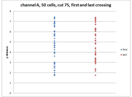
We have verified the method with simulations in type A channel for 20, 50, and 100 RBC, and in channel C for 50 RBC. Our analysis originated from the cell transitions at the 4 cut positions mentioned in Section 3. For each of the cells, we captured its position at the first and at the last transition trough each of the cutting positions. Thus, we obtained a set of 20 (50, 100) positions of the first and the last cell transition positions at this particular
channel location. Assuming that the RBC trajectories are
stable, these sets should be statistically identical,
respectively very similar. On the contrary, if trajectories tend to change, for example, shift to "typical"
trajectories; we should monitor some statistical
"simplification" of data and the like.
With the perspective of using the methodology for other types of channels, we have used the distance (in the y-axis direction) of the cell’s centre from the border of the closest obstacle, as the analysed value of the cell
position, when passing through a series of obstacles (cutting positions 25 + k.100 μm and 75 + k.100 μm). We used the distance (in the y-axis direction) of the cell
centre from the channel boundaries to measure cell positions in the channel sections between the obstacle arrays (cutting positions 50 + k.100 μm and 100 + k.100
μm).
Fig. 8. For 100 cell in channel A and cutting position 25 + k.100 μm two datasets of distances for first and last crossing are depicted. The difference in their distribution is not clear visible
Fig. 9. For 50 cell in channel A and cutting position 75 + k.100 μm the distributions of distances for first and last crossing are much more similar but not visible without statistical analysis
To evaluate the statistical similarity of these data for
the first and last cell transition trough the cutting position, we used the standard Two-Sample
Kolmogor-Smirnov test. It tests the hypothesis that both sets of the
data come from the same (unspecified) distribution.
Overall, we compared pairs of data sets for 5
simulations and 4 cutting positions in each of them. In
accept the hypothesis that the data is from the same distribution. In 2 cases, however, this hypothesis could be rejected at a 5% level of significance, once at 10% level and 5 times on a not very typical but used for the analysis at 15% level. Based on these results, we consider the methodology to be sufficiently sensitive and ready to process and assess the stability of RBC trajectories in more complex channels designed for real use.
Tab. 1. Table with results of K-S testing. Logical value 0 indicates acceptance of hypothesis that both datasets are from the same distribution. In other cases we depict the significance level, on which the hypothesis can be refused.
5 RBC’s Trajectories Data Processing
for Various Geometries
Our task was to analyse the blood flow in the microfluidic devices regarding the behaviour of individual cells and the capture of cancer cells on the device columns. In the case where only the fluid is moving in the microfluidic device, we can illustrate its flow through the stream lines. These are different for the various layouts of columns that capture the CTCs. In the case of a homogeneous fluid that does not contain blood cells, we could predict the transition of the cancer cell better than in the case of non-homogenous fluid, such as blood that in addition to the blood plasma contains also red blood cells, white blood cells, blood platelets and other blood components. The movement of cancer cells in the fluid (without other blood cells), in the microfluidic devices, is used to find suitable chemical bonds for the capture of cancer cells, for example in the article [14]. However, this model does not consider the influence of other objects in the blood. The role of diagnostics is to detect the presence of CTC cells between the healthy cells in the blood. In our model, we use red blood cells that are modelled as elastic bodies with properties similar to real objects, not only in shape, size and weight, but also in their elasticity.
The elastic properties of the blood cells cause that their movement in a microfluidic device is not predictable with only the knowledge of the fluid stream lines. For the further development of the device, we are interested in the movement of the CTC cell in a
microfluidic device and the characteristics that will describe the behaviour of the blood cells in terms of their movement in the device. At this stage in the development of the simulation model, it is our role to identify such statistical characteristics of the model that will allow us to predict the trajectory and the nature of the cell movement. We would like to obtain different values of these characteristics for different device geometries and different hematocrit levels. On the contrary, if the simulations differ only by the initial blood cells seeding, but their hematocrit levels and the geometry of the device (as well as other parameters such as the total flow rate) will be the same, we would like to obtain same values of the characteristics.
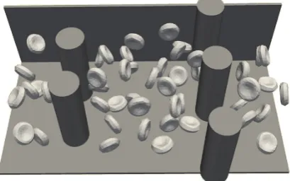
In this part of the paper we will look at the characteristics based on the mass properties of the whole set of blood cells in two different geometries, which are marked A and C, see Figure 10 and Figure 11, and by the number of used cells as A20, A50, A100, C50. The first experiments with these geometries are described in articles [11], [12], [10]. For our experiment, we used geometries with the same number of obstacles that were the same size, the only difference between these geometries was the distance of the obstacles. In each of the geometries, we did several simulations with different seedings.
Fig. 10. Geometry A with 50 randomly distributed red blood cells.
Fig. 11. Geometry C with 50 randomly distributed red blood cells.
The fluid flows in the direction of the x-axis, the channel width is in the y-axis direction and its height is in the direction of the z-axis as indicated in Figure 1.
5.1 Analysis of trajectories and output preparation for further statistical processing
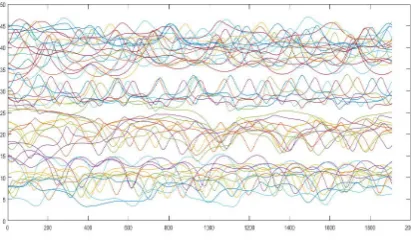
While examining a video from simulation, as well as from our previous analyses [13], it is clear that in each simulation steps, some cells move faster and others slower. Therefore, we cannot analyse only one of the coordinates when plotting and subsequently processing the trajectories of the blood cells. Figure 12 shows the simulation progress of X-coordinates of 50 blood cells centres, where the simulation step was used as an independent variable. The trajectories of moving blood cells, however, can be seen much better when the X-coordinate is chosen as the independent variable, as we can see in Figure 13.
Fig. 12. Geometry A50, the position of the Y-coordinates of the cells’ centre at each step of the simulation.
Fig. 13. Geometry A50, the position of the Y-coordinates of the cells’ centre depending on X-coordinate.
In Figure 14 we see the trajectories of moving cells in the direction of the Z-axis in relation to the X-coordinate. Since the obstacles in the microfluidic device do not change in this direction, the number of contacts with the obstacle that catches CTC cells, will not be dependent on the position in the Z-axis direction. Therefore, we do not include analysis of the Z-coordinate of the blood cells centres.
Fig. 14. Geometry A50, the location of the Z-coordinate of the cell centre in relation to X-coordinate.
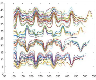
Figure 15 shows the trajectories of the moving cells in the Y-direction in relation to the X-coordinate for the geometry A for 50 cells. This is also done for the trajectories of 50 cells for geometry C in Figure 16.
Fig. 15. Geometry A50, two different seedings, Y-coordinate position in relation to X-coordinate
At various starting positions of the cells and their random rotation, we can find, for each geometry, typical trajectories as well as clusters of cells with the same typical patterns. In Figure 17, three seedings for geometry A are shown, and two seedings for geometry C are shown in Figure 18. In both cases, we synchronized the start of the trajectory only from the simulation step in which the cells reached the same value of the X-coordinate, corresponding to the end of the first crossing of the simulation channel.
Fig. 17. Geometry A50, three different seedings, the Y-coordinate position in relation to X-Y-coordinate. Values are shifted in the X-direction, to obtain the same starting position for all the cells.
Fig. 18. Geometry C50, two different seedings, the Y-coordinate position in relation to X-Y-coordinate. Values are shifted in the X-direction, to obtain the same starting position for all the cells.
For a smaller number of blood cells in the fluid, i.e., for a smaller hematocrit, there is a small number of interactions, whether between blood cells or between blood cells and obstacles in the microfluidic device. But even when simulating the flow of twenty blood cells in geometry A, in addition to the trend of copying, the study showed in the trajectory analysis of the site a slight change in the movement of the blood cells as can be seen in Figure 19.
Similarly, when analysing the flow of 100 cells in geometry A, on the one hand, we can see a strong trend to copy the trajectory. On the other hand, it is evident in Figure 20 that a lot of the cells move also in the Z-axis direction, or significantly slow down, which leads to smaller distance travelled in the X-axis direction (with the same number of time steps).
Fig. 20. Geometry A, 100 blood cells.
Distance profiles for each geometry and different amounts of cells are shown in the following charts. The distances are in ascending order. The values for the device with geometry A for 20, 50 and 100 cells are plotted on Figure 21, with two different initial seedings for 50 blood cells. For devices with geometry C, there are also two different initial seedings.
Fig. 21. X-axis distance profiles for different geometries and amounts of blood cells.
5.2. Principal component analysis and clustering of RBC centre trajectories
The processing of trajectories of the ensemble of the cells allow us to predict typical behaviour of blood cells and to estimate their trajectories based on the cluster in which the cell originates. The number of clusters and the variability of their patterns for the different microfluidic device geometries and for the different numbers of blood cells present in the device will be a characteristic used to optimize microfluidic devices. It is desirable that this characteristic will be the same for different initial
seedings in the same geometry and with the same number of blood cells, and differences will occur at different geometries and at different number of cells. Clusters for RBC centre trajectories are easily indefinable, in simulations that we have analysed so far, thus will not be further analyzed in this article. We will now focus on the Principal component analysis (PCA) method, which can help us not only distinguish between devices, but mainly can help us to determine the possible rate of success of the device capturing blood cells. In Figure 22, we can see differences in PCA results for the same geometry and different numbers of blood cells.
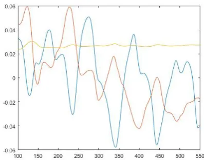
Fig. 22. Approximation of one of the trajectories using the first 4 principal components in geometry A. Gradually for 20, 50 and 100 cells.
are more blood cells, it is necessary to take more principal components for a better reconstruction of the trajectory, as seen in Figure 23 and Figure 24.
Fig. 23. Trajectory approximation of one of 50 cells using the first 9principal components in geometry A, seeding a.
Fig. 24. Trajectory approximation of one of 100 cells using the first 10 principal components in geometry A.
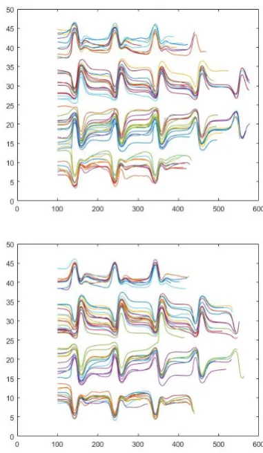
For each geometry and different number of RBC in them, in Figures 25, 26, 27, 28 and 29 we have always drawn three principal components. These determine the course of the most common trajectory and thus are a specific characteristic of the channel.
Fig. 25. The first three principal components for 20 cells in geometry A.
Fig. 26. The first three principal components for 50 cells in geometry A., seeding a.
Fig. 27. The first three principal components for 50 cells in geometry A, seeding b.
Fig. 29. The first three principal components for 50 cells in geometry C, seeding a.
In addition to the channel trajectory analysis, using the first three principal components, it is possible to interpret the PCA through trajectory reconstructions using the first principal components. Although the reconstructed trajectory differs from the actual trajectory, the error that will arise is in favour of the typical behaviour of all the blood cells. In the future, it will be useful to look mainly to the components of individual clusters that are visible from the trajectory even without a computer analysis. These PCA will allow us to predict the movement of the blood cell and later the cancer cell in the channel.
6 Applying of the investigated
characteristics to development of the
simulation model
In this article, we have presented a methodology to investigate the trajectories of the cells moving in microfluidic channels. We have verified that proposed methodology help us to recognize different modes of cell-movement in the channels. The proposed methodology will be than applied to several models of existing microfluidic channels. The next step of our study will be to evaluate the measure of collisions between the cells and the obstacles in the micro channel. Subsequently, the measures should be done with models containing a cancer cell(s). After that, we can compare the efficiency of tested microfluidic channels, eventually to propose an improvement of those channels.
References
1. S. Nagrath et al., Nature, 450, 1235–1239 (2007) 2. S. Hanasoge, R. Devendra, et al., Microfluidics and Nanofluidics, 18, 1195-1200 (2015)
3. S. Holm et al., Analytical Methods, 8.16, 3291-3300
(2016)
4. A. F. Sarioglu et al., Nature methods, 12.7, 685-691
(2015)
5. I. Cimrák, M. Gusenbauer, I. Jančigová, Computer
Physics Communications, 185, 900-907 (2014)
6. I. Cimrák, I. Jančigová, R. Tóthová, M. Gusenbauer,
Applications of Computational Intelligence in Biomedical Technology, 606, 1-28 (2015)
7. I. Cimrák, K. Bachratá, H. Bachratý, I. Jančigová, R.
Tóthová, M. Bušík, M. Slavík and M. Gusenbauer,
Communications, Scientific Letters of the University of Zilina, 18/1a, 13-20 (2016)
8. I. Cimrák, Computer Methods in Biomechanics and Biomedical Engineering, 1-6, 1525-1530 (2016)
9. M. Bušík, I. Jančigová, R. Tóthová, I. Cimrák, Journal
of Computational Science, 17, 370-376 (2016)
10. K. Kovalčíková, M. Slavík, Central European researchers journal, 3, 21-27 (2017)
11. M. Slavík, K. Bachratá, H. Bachratý and K. Kovalčíková, International Conference on Information and Digital Technologies 2017 (IDT) International Conference on. IEEE, 344-349 (2017)
12. H. Bachratý, K. Kovalčíková, K. Bachratá and M. Slavík, International Conference on Information and Digital Technologies 2017 (IDT) International Conference on. IEEE, 36-46 (2017)
13. K. Bachratá, H. Bachratý, M. Slavík,EPJ Web of Conferences, 143, (2016)