New solar modulation modeling of the galactic proton flux measured by the AMS02 and PAMELA experiments

New solar modulation modeling of the galactic proton flux

mea-sured by the AMS02 and PAMELA experiments

E. Fiandrini1,a, B. Bertucci1, N. Tomassetti1, and B. Khiali2

1_{Dipartimento di Fisica e Geologia, University of Perugia and INFN Perugia, Italy} 2_{INFN Perugia, Italy and ASI Space Science Data Center (SSDC), Roma, Italy}

Abstract.A thorough understanding of solar effects on the galactic cosmic rays is rel-evant both to infer the local interstellar spectrum characteristics and to investigate the dynamics of charged particles in the heliosphere. We present a newly developed numer-ical modulation model to study the transport of galactic protons in the heliosphere. The model was applied to the 27-day averaged galactic proton flux recently released by the PAMELA and AMS02 experiments, covering an extended time period from mid-2006 to mid-2017.

1 Introduction

Nearly all direct observations of Cosmic Rays (CRs) are made inside the heliosphere. As a result, the

CR spectrum observed at Earth can differ significantly from the Local Interstellar Spectrum (LIS) due

to many physical processes that modify the spectrum. This is particularly true for CRs with kinetic

energies below∼20 GeV, which can be efficiently diffused, curved and de-accelerated adiabatically

during their propagation from heliosphere to the Earth. The changes in the Galactic CR (GCR) inten-sities and energy spectra are related to the solar activity, and are referred to as CR solar modulation.

A thorough understanding of solar effects on the GCR propagation is therefore relevant both to infer

the LIS and to investigate the dynamics of charged particles in the heliosphere. It is also important for astronauts and the electronic components radiation hazard during long-duration missions.

The new precise data from AMS02 [1] and PAMELA [2] experiments offer a unique possibility to

study the solar modulation over a long period of time.

2 The proton model

Propagation in the heliosphere is described by the Parker’s equation[3]; ∂f

∂t =∇ ·[K· ∇f]−V~ · ∇f−< ~VD>·∇f + 1

3(∇ ·

~

V) ∂f

∂(lnp) (1)

Heretis the time, pis the CR particle momentum, ~V is the solar wind speed,VD~ is the averaged

guiding center speed for a pitch angle-averaged distribution functionfandKis the diffusion tensor. In

this work, a 2D numerical integration with∂/∂t=0 is made using a Stochastic Differential Equation approach with a backward time integration, based on [4].

The heliosphere is a dynamic void in the local interstellar medium where Sun activity dominates.

In this work the heliosphere has a spherical symmetry with the boundary located at r=122 AU, where

local interstellar spectrum is given as boundary condition, with the termination shock at r=85 AU

and the Earth position at r=1 AU in the equatorial plane. The Heliospheric Magnetic Field (HMF) is

wounded up in a modified Parker’s spiral [5, 6], as

B=B0( 1AU

r )

2 s

1+tan2(ψ)+₍rδ(θ) r

)2 ₍₂₎

whereB0 is the HMF value at Earth position, r is the Sun radius and δ(θ) = 8.7×10−5/sin(θ)

if θ < 1.7o _{or θ > 178}o _{and= 0 otherwise. A major corotating structure of importance to CR} modulation is the wavy Heliospheric Current Sheet (HCS), which divides the solar magnetic field

into hemispheres of opposite polarity. The HCS is parametrized by using its tilt angleαand is well

correlated to solar activity. The waviness of the HCS is one of the best proxy for solar activity relevant to CR modulation and is widely used in numerical approaches. The tilt angle has been observed at the Wilcox solar observatory since 1976.

Solar wind velocity is radially directed from close to the Sun, up to the inner heliosheath. During periods of minimum solar activity the flow is latitude dependent, changing from an average of 450

kms−1_{in the equatorial plane to 800 kms}−1_{in the polar regions. This significant effect disappears with}

increasing solar activity, when the average speed is∼400 kms−1 _{at all the latitudes. The latitudinal}

dependence of the solar wind speed is parametrized as in [7] and was made dependent on the solar activity by increasing the polar angle at which the solar wind speed changes from slow to fast as a function of the tilt angle.

Diffusion is described by a diagonal diffusion tensor with three diffusion coefficients, namely

parallel diffusion K||, the transverse radial,K⊥r, and transverse polar diffusion coefficient,K⊥θ. The

parallel diffusion can be computed using quasi linear theory [8]. The diffusion coefficient parallel to

the background field,K||, was parametrized as in [10]

K||=K0β B0

B _R

0 R

a"(R/R

0)h+(Rk/R0)h

1+(Rk/R0)h

#(b−a)/h

(3)

withβ= v/c, the ratio of the particle’s speed to the speed of light. K0 is a constant in units of

1023 _cm2_s−1_{, withR}

0 = 1 GV, B the HMF magnitude and B0 the local field value, such that the

units are inK0. Hereaandbare a power indexes that determine the slope of the rigidity dependence,

respectively, below and above a rigidity with the valueRk, whereash=3.0 determines the smoothness

of the transition. The valueRkdetermines the rigidity where the break in the power law occurs. The

parametersK0,a,bdepend on the solar activity, therefore vary in time and are free parameters that

can be used to fit measured CR flux at a given epoch. Perpendicular diffusion in the radial direction is

parametrized asK⊥r =0.02×K||, which a widely used assumption [9], while the polar perpendicular

diffusion was parametrized as K⊥θ = 0.02×g(θ)×K||, whereg(θ) is a function that enhances the

diffusion by a factor d=3 near the poles, as defined by Eqn. (8) in [10].

The motion in the large-scale average HMF is given by pitch-angle averaged velocityVD. In this

2D modeling, the HCS is described as a region with an extension that depends on the rigidity of CR particles and on the value of the tilt angle. In this approach, the drift velocity is given by

<VD>= f(θ)∇ ×      KA

~ B B      +

∂f(θ) ∂θ

! KA

r ~eθ× ~ B

The first term describes the gradient and curvature drifts, while the second one describes the motion

in the region affected by the HCS. f(θ) is a function that describes the transition between the regions

inside and outside the HCS, given in [6],~eθis the unit vector along the polar direction andKAis the

anti-symmetric part of the diffusion tensor [11], given by

KA =KA0 Q

|Q|

βR B

" _(R/RAk)2

1+(R/RAk)2

#

(5)

HereQis the CR charge,RAkis the break inKAandKA0=1. The local interstellar spectrum (LIS) of

galactic CR is an input for any modulation models. Fluxes are assumed isotropically distributed at heliosphere boundary, in a steady-state configuration. In the current model the proton LIS flux that was used is taken from [13].

2.1 Application to AMS02 and PAMELA data

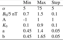
The numerical model was applied to the Bartel-rotation averaged AMS02 data from May 2011 to May 2017 [1] and to the Bartel-rotation averaged PAMELA data from June 2006 to January 2014 [2]. The model has six free parameters that can be varied to fit the measured data sets. They are: tilt angle α(t), HMF at EarthB0(t), the HMF polarityA(t), the parallel diffusion normalization coefficientK0(t),

the two spectral indexes of the diffusion coefficient,a(t) andb(t). The first three define the average

status of heliosphere at a given epoch, the last three fit the data sets and define the modulation of CR

at the same epoch. The breakRk is fixed atRk=3 GV andRAk=0.3 GV, since it was seen that can

be treated as constant in time. As a first approximation, to take into account the time-varying status of the heliosphere, we take the averaged tilt angle and HMF over a time period of 1 year preceding the selected BR, using a Backward Moving Average (BMA). To fit the measured data sets of CR of

AMS02 and PAMELA, a six dimensional discrete grid of the model parameters vector~q=(α,B0,A,

K0,a,b) was built with the parameters values shown in the Table 1.

Table 1.Model parameters ranges and step used to build the proton model flux grid.

Min Max Step

α 5 75 5

B0/5 nT 0.7 1.5 0.1

A -1 1 1

K0 0.1 0.9 0.1

a 0.45 1.4 0.05

b 0.45 1.65 0.05

For each of the 1.215×106_{points in the grid, a proton fluxJm(E, ~q) was simulated.}

Then, for each data setJd(E,t), aχ2_{was defined as}

χ2_(~q)=X i

_Jd(Ei,_t)−Jm(Ei, ~_q)2

σ2_(Ei,t) (6)

The errors are given byσ2_{(Ei,t) = σ}2

d(Ei,t)+σ 2

S DE(Ei,t). Hereσ 2

d(Ei,t) are the experimental

errors fori-th energy bin andσ2

S DE(Ei,t) are the errors due to the limited statistics of the Stochastic

Differential Equation (SDE) MonteCarlo approach and the uncertainties in the LIS flux. These errors

Low Index a

χ

2   mi

n

/(

Nd

of

– 1)

a_best  =  0.93  ±  0.15  

Low Index a

•   •  

•  

•   _{•   •   •}   •  

•  •  •  

•   •   •  

•   •   •  

•   _•   •  

χ

2     mi

n

/(

Nd

of

– 1)

(a) (b)

Figure 1.(a) Distribution of theχ2_{of the parametera. The black dots indicate theχ}2

mincurve. (b)χ

2

mincurve for

the same data set as in (a).xbestand errors are shown as solid and dashed lines, respectively.

at a given epoch, defined as the timet of the beginning of the corresponding BR, the first three

parameters,α(t),B0(t) and A(t) fix the average status of the heliosphere. Forx=K0(t),a(t) andb(t)),

the minimum chi-squared curve,χ2_min(x), is found, regardless of the values of all the other parameters,

as shown in Figure 1a for the spectral index below the breakafor one data set, where theχ2_min(x)

is represented by the black dots. Then, an interpolation is done on theχ2_min(x) to find its miminum

and the value of the parameter x at minimum,xbest. The errors on the parameters are estimated as

σx=max(|x−−xbest|,|x+−xbest|), wherex±is the parameter value such thatχ2min(x±)=χ2min(xbest)+1

above and belowxbest, as shown in 1b, where the solid line indicates xbest and the dashed lines x±.

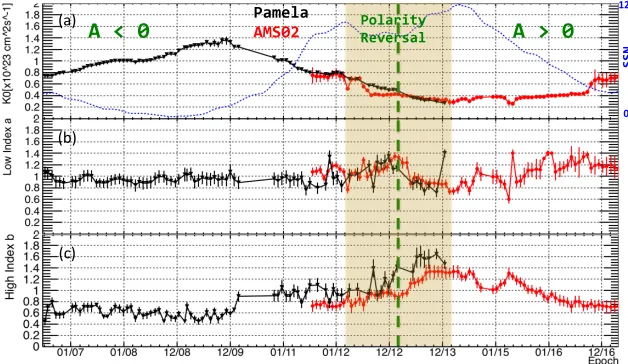
The model was applied to the Bartel-Rotation averaged proton fluxes measured by the PAMELA and AMS02 experiments [1, 2]. The data time-series cover the solar minimum from 2006 to 2009, the

ascending phase to solar maximum, occurred on∼February 2013, when the Sun polarity A reversed,

and the following descending phase until May 2017. The comparison to the data,P|Jd−Jbest|

σ , shows

that the difference between any data set and the corresponding best flux model are all well below 1. In

Figure 2 are shown the model parametersK0,aandbas a function of time for the data sets of AMS02

and PAMELA. It is clearly visible a correlation to the solar activity measured by the averaged Sun Spot Number (SSN) with a time lag between the SSN and the model parameters. To find the time lag

between the model parameters and the SSN we compareK0(t) with SSN(t -∆t) varying∆tand find

the∆tthat maximizes the correlation. It turns out to be∆t =1.04±0.1 years. K0is anti-correlated

with SSN when time lag is taken into account, the slopesaandbare less clearly correlated with SSN

but a variation can be seen between solar max and solar min.

3 Conclusions

A new modeling of the proton flux has been implemented. It successfully describes AMS02 and PAMELA data covering 11 years of CR measurements. A clear correlation between solar activity and CR modulation is found. The model array can be used to find the modulation parameters at any epoch.

References

Fiandrini   1  

A  <  0  

A  >  0  

AMS02  

 SSN  

120  

0   (a)  

(b)  

(c)  

Figure 2. Results for (a)K0, (b) spectral indexaand (c) spectral indexbfor all the data sets as a function of

time. Dotted line in (a) displays the averaged SSN.

[3] Parker, E. N. 1965, Planet. Space Sci., 13, 9 [4] Kappl, Comp. Phys. Comm. 207 (2016) 386?399 [5] Parker, E. N. 1958, ApJ, 128, 664

[6] Bobiket al.The Astroph. J., 745:132 (21pp), 2012

[7] Potgieter, M. S., Vos, E. E., Boezio, M., et al. 2014, SoPh, 289, 391 [8] Jokipii, J. R. 1966, ApJ, 146, 480

[9] le Roux, J. A. , Fichtner, H. 1999, J. Geophys. Res., 104, 4709

[10] M.S. Potgieter et a., Solar Phys (2014) 289:391?406 DOI 10.1007/s11207-013-0324-6