array of 507 plastic scintillation counters on a 1.2 km square grid and fluorescence detectors at three stations overlooking the sky above the air shower array. The experiment and its recent measurements - spectrum, composition, and anisotropy - is reviewed. Recently the construction of the TA Low energy Extension (TALE) detector, which consists of an additional fluorescence detector and an infill array, was finished. TALE lowers the energy threshold of TA down to 4 PeV. We are also constructing the TAx4 detector to increase statistics in particular at the highest energies. The current status and the future prospects of these new TAx4 experiments is reported.
1 Introduction
Telescope Array (TA) is an observatory for ultra high en-ergy cosmic rays in the northern hemisphere. Operating TA together with the TA Low energy Extension (TALE) detectors, we archive a vary wide target energy range from
1016 to 1020 eV. The next section is a briefly
introduc-tion of the Telescope Array experiment, such as our de-tectors and analysis. In section 3, I will report recent re-sults on the energy spectrum, chemical composition and anisotropy studies. Section 4 is an introduction and status
report of on-going extension projects called TA ×4 and
TALE.
2 The Telescope Array Detectors
The TA site is located in the desert about 1400 m above sea level centered at 39.3◦N and 112.9◦W in Millard county, Utah, USA, about 200 km southwest of Salt Lake City. A control center to support operations of the TA, TALE and
TA×4 instruments is in the city of Delta located near the
northeast side of the TA SD array.
Figure 1 is a map of the TA site, and the dots and markers indicate the locations of detectors. Figure 2 shows some of the infrastructure. The TA surface detector (SD) array consists of 507 scintillation detectors of 3 square me-ter size deployed with 1.2 km spacing. The coverage area
by the SD array is about 700 km2. The sky above the array
is observed by 38 fluorescence detectors (FDs), installed in three stations which are called Middle Drum (MD), Black Rock Mesa (BRM) and Long Ridge (LR) stations. The ar-rows in Figure 1 indicate the border of the field of view (FOV) of each FD station. The telescopes in the MD
sta-tion were arranged to view 120◦in azimuth and 3◦−33◦in
elevation. Comparing with the MD station, the azimuthal ∗e-mail: [email protected]
Figure 1.The map of the TA site. The labeled black dots indicate the location of SDs, and the green open square is the positions of the FD stations. The three open orange markers indicate the location of the communication towers.
FOV of the BRM and the LR stations is narrow and 108◦.
At the center of the array, there is the central laser facil-ity (CLF) used for the calibrations of FDs. The distance between the CLF and each FD station is about 20 km.
Figure 2. Pictures of the four FD stations and of the telescopes and cameras in the stations.
2.1 Fluorescence Detectors
The MD station has 14 telescopes, each of which consists of a refurbished telescope used in HiRes-I [1], a camera comprising 256 PMTs. Each telescope unit uses
sample-and-hold electronics with a 5.6µs gate.
Just beside the MD station, there is the TALE-FD sta-tion which has ten refurbished HiRes-II [1] telescopes ob-serving higher elevation angles which means measuring lower energies, than TA. These are the refurbished HiRes-II telescopes. A camera of 256 pixels is placed at the focal plane of the mirror. Each pixel covers a one degree cone
in the sky, and each camera has a FOV of 16◦in azimuth
by 14◦in elevation. The PMT signals are recorded by a 10
MHz FADC readout system with an 8-bit resolution. Ana-log sums over rows and columns of pixels, also sampled at 8-bits, allow recovery of saturated PMTs in most cases.
The systems in the LR and the BRM stations are actly the same, and it was newly designed for the TA ex-periment [2]. Each station has 12 telescopes, and each
telescope has 256 PMTs focused onto a 6.8 m2mirror for
light collection. Each PMT’s analog signals are digitized by FADC electronics which employ 12 bit digitizers oper-ating at 40 MHz. Before storage to the DAQ, four digital samples are summed to provide an equivalent 14 bit, 10 MHz sampling rate providing a time resolution of 100 ns.
The process of analysis consists of four steps: PMT selection, shower geometry reconstruction, reconstruction of longitudinal shower profile and quality cuts. An FD monocular plane fitting procedure determines the geom-etry of the air shower track relative to the observing FD. At first the shower-detector plane (SDP) normal vector is found from the number of tubes along the shower track, the pointing directions and the tube signals of each tube in the SDP. In the monocular reconstruction, once the SDP is known, the shower impact parameter and the SDP an-gle are calculated by comparing the observed tube trig-ger times and the expected trigtrig-ger times. Using the in-formation from the two stations simultaneously allows the "stereo reconstruction". For the stereo analysis the shower geometry is determined primarily by finding the intersec-tion of the two SDPs. The other idea called "hybrid
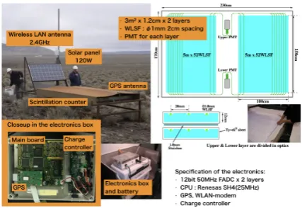
re-Figure 3.Pictures of a surface detector and electronics.
construction" is the use of timing information from one or more SDs in addition to the FD tube timings. The SD tim-ing at which the shower plane crosses the ground gives an “anchor” in the conventional FD timing fit. The stereo or hybrid reconstructions significantly improve the accuracy in shower geometry determination compared to that of the FD monocular mode.
Once the shower geometry is determined, the shower profile including the depth of shower maximum (Xmax) determined using the light profile observed by the FDs by the inverse Monte Carlo method, and then finally the pri-mary energy is found by integrating the shower profile.
2.2 Surface Detector Array
The SD array consists of 507 detector units, which were deployed in a square grid with 1.2 km spacing to cover
a total area of approximately 700 km2. Each surface
de-tector has a scintillation counter, a solar panel, a wireless LAN and GPS antennas, and a controlling electronics and a battery behind the solar panel on a steel platform (see Fig. 3). The scintillation counter consists of two layers of plastic scintillator. Each layer of scintillator has an area of
3 m2and a thickness of 1.2 cm. Scintillation light is
col-lected through 104 wavelength-shifting (WLS) fibers, and both ends of the fibers from a layer are bundled together and connected to a PMT. The controlling electronics con-sists of 12bit 50MHz FADCs, a CPU, a GPS module, a wireless LAN modem and a charge controller.
Figure 2. Pictures of the four FD stations and of the telescopes and cameras in the stations.
2.1 Fluorescence Detectors
The MD station has 14 telescopes, each of which consists of a refurbished telescope used in HiRes-I [1], a camera comprising 256 PMTs. Each telescope unit uses
sample-and-hold electronics with a 5.6µs gate.
Just beside the MD station, there is the TALE-FD sta-tion which has ten refurbished HiRes-II [1] telescopes ob-serving higher elevation angles which means measuring lower energies, than TA. These are the refurbished HiRes-II telescopes. A camera of 256 pixels is placed at the focal plane of the mirror. Each pixel covers a one degree cone
in the sky, and each camera has a FOV of 16◦ in azimuth
by 14◦in elevation. The PMT signals are recorded by a 10
MHz FADC readout system with an 8-bit resolution. Ana-log sums over rows and columns of pixels, also sampled at 8-bits, allow recovery of saturated PMTs in most cases.
The systems in the LR and the BRM stations are actly the same, and it was newly designed for the TA ex-periment [2]. Each station has 12 telescopes, and each
telescope has 256 PMTs focused onto a 6.8 m2mirror for
light collection. Each PMT’s analog signals are digitized by FADC electronics which employ 12 bit digitizers oper-ating at 40 MHz. Before storage to the DAQ, four digital samples are summed to provide an equivalent 14 bit, 10 MHz sampling rate providing a time resolution of 100 ns.
The process of analysis consists of four steps: PMT selection, shower geometry reconstruction, reconstruction of longitudinal shower profile and quality cuts. An FD monocular plane fitting procedure determines the geom-etry of the air shower track relative to the observing FD. At first the shower-detector plane (SDP) normal vector is found from the number of tubes along the shower track, the pointing directions and the tube signals of each tube in the SDP. In the monocular reconstruction, once the SDP is known, the shower impact parameter and the SDP an-gle are calculated by comparing the observed tube trig-ger times and the expected trigtrig-ger times. Using the in-formation from the two stations simultaneously allows the "stereo reconstruction". For the stereo analysis the shower geometry is determined primarily by finding the intersec-tion of the two SDPs. The other idea called "hybrid
re-Figure 3.Pictures of a surface detector and electronics.
construction" is the use of timing information from one or more SDs in addition to the FD tube timings. The SD tim-ing at which the shower plane crosses the ground gives an “anchor” in the conventional FD timing fit. The stereo or hybrid reconstructions significantly improve the accuracy in shower geometry determination compared to that of the FD monocular mode.
Once the shower geometry is determined, the shower profile including the depth of shower maximum (Xmax) determined using the light profile observed by the FDs by the inverse Monte Carlo method, and then finally the pri-mary energy is found by integrating the shower profile.
2.2 Surface Detector Array
The SD array consists of 507 detector units, which were deployed in a square grid with 1.2 km spacing to cover
a total area of approximately 700 km2. Each surface
de-tector has a scintillation counter, a solar panel, a wireless LAN and GPS antennas, and a controlling electronics and a battery behind the solar panel on a steel platform (see Fig. 3). The scintillation counter consists of two layers of plastic scintillator. Each layer of scintillator has an area of
3 m2and a thickness of 1.2 cm. Scintillation light is
col-lected through 104 wavelength-shifting (WLS) fibers, and both ends of the fibers from a layer are bundled together and connected to a PMT. The controlling electronics con-sists of 12bit 50MHz FADCs, a CPU, a GPS module, a wireless LAN modem and a charge controller.
The process of analysis for SD array data consists of three steps (see Fig. 4). At first a time fit of shower arrivals at SDs is performed to determine the geometry of the cos-mic ray air shower. The lateral distribution of charged par-ticle densities at the SDs is fit using the AGASA lateral distribution function [3, 4] to determine S800, the density of shower particles at a lateral distance of 800 m from the air shower axis. The primary energy of the cosmic ray is estimated by using a look-up table in S800 and the shower zenith angle. The table is obtained by a large statistics MC simulation using CORSIKA and the QGSJET II-03 hadronic model. Finally, the reconstructed energy by the SD analysis is scaled to the energy measured by the TA
Figure 4.The process of analysis for SD array data
Figure 5.The nine year spectrum measured by the TA SD array [6]
FDs, which is determined using calorimetric detection of an air shower energy deposition in the atmosphere with less hadronic interaction dependence than the SD [5].
3 Recent Results
3.1 Energy spectrum and related studies
Figure 5 is the nine year spectrum measured by the TA SD array, and the data points fit to a broken power law [6].
There are two breaks, the ankle at 1018.69eV and a cutoff
at 1019.81eV. The significance of the existence of the cutoff
is about seven sigma.
The Auger-TA spectrum working group showed a comparison between Auger and TA SD spectra, which do not overlap each other by about 10% energy shift. How-ever, this shift is well within the stated systematic energy scale uncertainties by Auger 14% and TA 21%. When the Auger energies are raised by 5.2% and TA energies lowered by 5.2%, as shown in Figure 6(a), the fluxes by
two experiment well overlap below 1019.4 eV.
Neverthe-less, the two fluxes do not overlap each other at energies
higher than 1019.4 eV. However, if we use data only from
the common declination band, that is from -15.9 degree to
Figure 6.A comparison between TA SD full sky spectrum with energies scaled by –5.2% and Auger SD full sky spectrum with energies scaled by+5.2% [7]. (a) is a comparison of the full sky spectra, and (b) is a comparison of the spectra for the common declination band.
Figure 7.TALE cosmic rays energy spectrum measured with 22 months of data [8].
24.8 degree, we can see a better agreement between Auger and TA as shown in Figure 6(b).
Figure 7 is the two year spectrum in the lower energy
range, from 1015.3 eV to 1018 eV, measured by the TALE
FDs, and the data points fit to a broken power law [8].
There are two breaks, a break at 1016.22 and the second
knee at 1017.04eV. We note that since the estimation of
ex-posure strongly depends on the chemical composition in particular in the lower energy region, the energy spectrum also depends on an assumed chemical composition. For Figure 7 a mixed primary composition representing the re-constructed Xmax distribution is assumed. The gray band indicates the size of the systematic uncertainties.
3.2 Chemical Composition
FIgure 8 is the mean Xmax, < Xmax > , as a
Figure 8. Mean Xmax as a function of energy as observed by TA in BRM and LR hybrid mode over 8.5 years of data collection [9].
analysis. Reconstructed Monte Carlo of four different pri-mary species generated using the QGSJet II-04 hadronic model are shown for comparison [9]. Within systematic
uncertainties,<Xmax>of the data is in agreement with
QGSJet II-04 protons and helium for nearly all energy bins. There is a clear separation between the region of sys-tematic uncertainty and heavier elements such as nitrogen and iron.
The reconstructed Xmax distribution for a single el-ement, such as QGSJet II-04 protons is sampled accord-ing to the same number of events recorded in the data for
a given energy bin. < Xmax >and the standard
devi-ation of Xmax distribution, σ(Xmax), of the energy are
calculated and recorded for this sample. This procedure is
then repeated 5000 times. The distribution of<Xmax>
andσ(Xmax) is used to calculate the 68.3%, 90%, and
95% confidence intervals. The entire < Xmax > and
σ(Xmax) calculated by this method is then plotted as a
2-dimensional distribution along with the computed con-fidence intervals. This procedure is repeated for the other three chemical elements used in the analysis. Figures 9 shows this measurement for all observed energy bins. The
< Xmax >and σ(Xmax) of the data observed in each
energy bin is also recorded as a single red star. Addi-tionally, the statistical, systematic, and combined statis-tical and systematic error bounds are marked around the data. Figures 9(a) – 9(f), corresponding to the energy range 1018.2−1018.8eV showσ(Xmax) of the data to
re-semble QGSJet II-04 protons, and<Xmax>of the data
falls within the 68.3% confidence interval of the proton distributions within the data’s systematic uncertainty.
Figure 9(g), corresponding to the energy range 1018.8−
1018.9 eV, shows that the 68.3% confidence intervals of
QGSJet II-04 proton and helium both fall within the bounds of the systematic uncertainty of the data. In Figure 9(h), corresponding to the energy range 1018.9−1019.0eV,
σ(Xmax) of the data fluctuates up from the previous
en-ergy bin and the systematic error bounds of the data falls within the 68.3% confidence interval of protons. In Figure 9(i), the 68.3% confidence intervals of both proton and
he-Figure 9. Measurements of data and QGSJet II-04 Monte Carlo
<Xmax>andσ(Xmax). Each Monte Carlo chemical element shows the 68.3% (blue ellipse), 90% (orange ellipse), and 95% (red ellipse) confidence intervals.
Figure 10. Significance map from 9 yr TA-SD events E>57 EeV with 25◦oversampling radius.
lium fall within the bounds of the systematic uncertainty of the data. Figures Figure 9(j) and 9(k) show that within the data’s systematic uncertainty the data may resemble QGSJet II-04 proton, helium, or nitrogen.
3.3 Arrival Direction Distributions
In the highest energy set with E>57 EeV collected
dur-ing the first 5 years of the TA operation, a concentration of
events has been observed in the circle of radius 20◦around
the direction RA=146.7◦, DEC=43.2◦[10]. The number
of events has been almost doubled now, and we scanned
the oversampling radius from 15◦ to 35◦ with 5◦
inter-val. We found the maximum significant excess appears at RA=144.3◦, DEC=40.3◦with the 25◦oversampling ra-dius as shown in Figure 10. The statistical significance is
5.1σ, and the probability of such a hotspot appearing by
Figure 8. Mean Xmax as a function of energy as observed by TA in BRM and LR hybrid mode over 8.5 years of data collection [9].
analysis. Reconstructed Monte Carlo of four different pri-mary species generated using the QGSJet II-04 hadronic model are shown for comparison [9]. Within systematic
uncertainties,<Xmax>of the data is in agreement with
QGSJet II-04 protons and helium for nearly all energy bins. There is a clear separation between the region of sys-tematic uncertainty and heavier elements such as nitrogen and iron.
The reconstructed Xmax distribution for a single el-ement, such as QGSJet II-04 protons is sampled accord-ing to the same number of events recorded in the data for
a given energy bin. < Xmax >and the standard
devi-ation of Xmax distribution, σ(Xmax), of the energy are
calculated and recorded for this sample. This procedure is
then repeated 5000 times. The distribution of<Xmax>
andσ(Xmax) is used to calculate the 68.3%, 90%, and
95% confidence intervals. The entire < Xmax > and
σ(Xmax) calculated by this method is then plotted as a
2-dimensional distribution along with the computed con-fidence intervals. This procedure is repeated for the other three chemical elements used in the analysis. Figures 9 shows this measurement for all observed energy bins. The
< Xmax >and σ(Xmax) of the data observed in each
energy bin is also recorded as a single red star. Addi-tionally, the statistical, systematic, and combined statis-tical and systematic error bounds are marked around the data. Figures 9(a) – 9(f), corresponding to the energy range 1018.2−1018.8eV showσ(Xmax) of the data to
re-semble QGSJet II-04 protons, and<Xmax>of the data
falls within the 68.3% confidence interval of the proton distributions within the data’s systematic uncertainty.
Figure 9(g), corresponding to the energy range 1018.8−
1018.9 eV, shows that the 68.3% confidence intervals of
QGSJet II-04 proton and helium both fall within the bounds of the systematic uncertainty of the data. In Figure 9(h), corresponding to the energy range 1018.9−1019.0eV,
σ(Xmax) of the data fluctuates up from the previous
en-ergy bin and the systematic error bounds of the data falls within the 68.3% confidence interval of protons. In Figure 9(i), the 68.3% confidence intervals of both proton and
he-Figure 9. Measurements of data and QGSJet II-04 Monte Carlo
<Xmax>andσ(Xmax). Each Monte Carlo chemical element shows the 68.3% (blue ellipse), 90% (orange ellipse), and 95% (red ellipse) confidence intervals.
Figure 10. Significance map from 9 yr TA-SD events E>57 EeV with 25◦oversampling radius.
lium fall within the bounds of the systematic uncertainty of the data. Figures Figure 9(j) and 9(k) show that within the data’s systematic uncertainty the data may resemble QGSJet II-04 proton, helium, or nitrogen.
3.3 Arrival Direction Distributions
In the highest energy set with E>57 EeV collected
dur-ing the first 5 years of the TA operation, a concentration of
events has been observed in the circle of radius 20◦around
the direction RA=146.7◦, DEC=43.2◦ [10]. The number
of events has been almost doubled now, and we scanned
the oversampling radius from 15◦ to 35◦ with 5◦
inter-val. We found the maximum significant excess appears at RA=144.3◦, DEC=40.3◦with the 25◦oversampling ra-dius as shown in Figure 10. The statistical significance is
5.1σ, and the probability of such a hotspot appearing by
chance in an isotropic cosmic-ray sky is 3.0σ.
Figure 11. This map shows the overview of the TA site. Each green circle in the northeast and southeast corresponds to the planned location of each TAx4 SD. The spacing of TAx4 SD is 2.08 km. The red circle in the west shows the location of TA SD. The spacing of TA SD is 1.2 km. The 2 fan shapes drawn with black lines describe the expected field of view from TAx4 FDs. Four telescopes of FD will be built in the north Middle Drum site and 8 telescopes of FD will be built in the south Black Rock site. The overlap of the locations of SD and the field view of FD enables SD and FD hybrid observation.
4 Extension of Telescope Array
4.1 TA×4
New SDs and FDs are planned to be constructed for the TAx4 experiment to cover 4 times larger area than TA,
about 3000km2, to observe cosmic rays especially with
the highest energies using high statistics (Fig. 11). This project is expected to clarify not only the source of the hotspot but also the energy spectrum and the composition
at the highest energies. The five-year proposal for TA×4
SD was accepted in the spring of 2015. The proposal for constructing 2 FD stations was also accepted in 2016. In our plan, 500 SDs are going to be made and deployed with 2.08 km spacing. After 3 years construction work, 180 SDs in Utah and the next 60 are to be prepared at ICRR and SKKU in 2018. For two FD stations with refur-bished twelve HiRes telescopes, telescopes and electronics were prepared at the University of Utah, and the northern stations had been installed and observed the first light in 2018. The site construction is underway at the southern site.
Figure 12. A map of the TA experiment site and a close up of TALE site are shown.
4.2 TA Low energy Extension (TALE)
The Telescope Array Low-energy Extension (TALE) ex-periment is a hybrid air shower detector for observation of air showers produced by very high energy cosmic rays
above 1016.5 eV. TALE is located at the TA site (see
Fig. 12). TALE has a SD array made up of 80 scintillation counters (40 with 400 m spacing, 40 with 600 m spacing) and a FD station consisting of ten FD telescopes located at the TA Middle Drum station. TALE-FD full operation started in 2013. The deployment of 80 SDs and the
instal-lations of DAQ/control electronics had been completed by
February 2018.
Acknowledgements
tional Trust Lands Administration (SITLA), U.S. Bureau of Land Management (BLM), and the U.S. Air Force. We appreciate the assistance of the State of Utah and Fillmore offices of the BLM in crafting the Plan of Development for the site. Patrick Shea assisted the collaboration with valuable advice on a variety of topics. The people and the officials of Millard County, Utah have been a source of steadfast and warm support for our work which we greatly
[4] M. Takeda, Astropart. Phys.19, 447(2003)
[5] T. Abu-Zayyad et al., ApJL768, L1(2013)
[6] J. N. Matthews, ICRC2017, CRI172(2017) [7] D. Ivanov, ICRC2017, CRI231(2017)
[8] R. U. Abbasi et al., ApJ, in press; arXiv: 1803.01288(2018)
[9] R. U. Abbasi et al., ApJ858, 76(2018)

![Figure 8.Mean Xmax as a function of energy as observed byTA in BRM and LR hybrid mode over 8.5 years of data collection[9].](https://thumb-us.123doks.com/thumbv2/123dok_us/8008700.1331038/4.595.67.278.83.220/figure-mean-xmax-function-energy-observed-hybrid-collection.webp)

