631 | P a g e
STUDY ON EFFECT OF STANDARD DEVIATION OF
SEDIMENTS ON HYDRAULIC CONDUCTIVITY
Janmeet Singh
1
ME Student Civil Engineering, PEC University of Technology, Chandigarh, (India)
ABSTRACT
In the field of hydrogeology it is important to know how easy water can move through porous media . Hydraulic conductivity is one of the most important physical properties of soil which governs the quantitative evaluation of groundwater resources. It is highly dependent upon aquifer properties and flow regime. It is desirable to predict the hydraulic conductivity value of same shape group particles of different sizes and mixed randomly for a knowledge of their statistical size distribution. To investigate the variation of Hydraulic conductivity with respect to standard deviation, the present study has been conducted. The effect of standard deviation on hydraulic conductivity has been studied analytically as well as experimentally. The residuals and deviation of measured and estimated values of hydraulic conductivity have been measured.
Keywords
:
Hydraulic Conductivity , Standard Deviation , PermeameterI INTRODUCTION
The crisis of access to adequate and safe drinking, agricultural and livelihood activity has gained due attention in recent years as it grapples with the problem of water shortage in many of its regions. Due to rapid development, increasing population and inadequate distribution of water , the demand for this natural resources far outweighs its supply . All these considerations and other make it necessary to study the behavior of water through soil and to evaluate properties such as hydraulic conductivity (K) ,one of the most important parameters required for predicting the movement of water through soil . The percolation of fluids through porous media is an important phenomenon that occurs appreciably in many physical situations such as flow through aquifers and in situations where packing material is contained within structures like ground water extraction by drilling through the strata, cooling towers, sewage treatment plants and chemical reactors. The present study is an experimental work involving a study on effect of standard deviation on hydraulic conductivity .
II EXPERIMENTAL WORK
632 | P a g e
Figure 1 : Constant Head Permeameter 2.1 Experimental Equipment
The experimental equipment consists of the following items:
a) Permeameter
The constant head vertical flow type permeameter was used for hydraulic tests in this work. The main permeameter section consisted of a 10.16 cm internal diameter GI tube with a total length of 1.06 m and a test length of 46.5 cm.
b) Discharge measurement
The discharge was measured by volumetric method. The water was collected in a bucket for a certain period, which was recorded with a stopwatch and collected water was then measured with the help of a 2000 cc capacity glass jar. Volume of water collected at a particular duration will give the discharge.
c) Weighing balance
Electronic weighing balance were used for measuring the weight during specific gravity test
d) Pycnometer
I.S. pycnometer is used in the specific gravity test.
e) Manometer
To cover the desired range of flow, two types of manometer were used: (i) Air-water manometer
(ii) Paraffin water manometer
f) Thermometer
633 | P a g e
g) Source of supply
The permeameter receives its water supply from an overhead tank at a height of 2.65 m above the permeameter outlet. The tank receives its supply from a recirculating tank so that a constant head is maintained in the overhead tank.
h) Oven
Oven was used to dry out the soil samples collected from different boreholes before performing the sieve analysis.
2.2 Materials Used and media preparation
Natural sand samples were collected from different boreholes exhibits different grain size distribution curve were used in the present study . After precalculated Geometric standard deviation of each sample , media was prepared by mixing the particles around median diameter in order to obtain the required standard deviation .Table 1 to 6 illustrates the value of standard deviation which was used in this study
Table 1 Grain size diameter and standard deviation for sand sample 1
Sample No. d50 (cm) Standard deviation (σ)
1 0.0425 Uniform
1 0.0425 1.367
1 0.0425 1.554
1 0.0425 2.019
1 0.0425 2.424
Table 2 Grain size diameter and standard deviation for sand sample 2
Sample No. d50 (cm) Standard deviation (σ)
2 0.05 Uniform
2 0.05 1.41
2 0.05 1.65
2 0.05 2.31
2 0.05 2.93
Table 3 Grain size diameter and standard deviation for sand sample 3
Sample No. d50 (cm) Standard deviation (σ)
634 | P a g e
3 0.06 1.37
3 0.06 1.59
3 0.06 2.257
3 0.06 2.82
Table 4 Grain size diameter and standard deviation for sand sample 4
Sample No. d50 (cm) Standard deviation (σ)
4 0.0425 Uniform
4 0.0425 1.21
4 0.0425 1.4
4 0.0425 2.05
4 0.0425 2.83
Table 5 Grain size diameter and standard deviation for sand sample 5
Sample No. d50 (cm) Standard deviation (σ)
5 0.03 Uniform
5 0.03 1.29
5 0.03 1.63
5 0.03 2.39
5 0.03 2.61
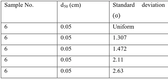
Table 6 Grain size diameter and standard deviation for sand sample 6
Sample No. d50 (cm) Standard deviation (σ)
6 0.05 Uniform
6 0.05 1.307
6 0.05 1.472
6 0.05 2.11
6 0.05 2.63
2.3 Experimental Procedure
635 | P a g e
a) Sieve analysis tests
Six samples were used in the present investigation which were collected from six different boreholes of different regions .The sediment samples were sieved mechanically through the various sieves sizes ranging from 2.36mm ,1.18mm , 850μ ,600 μ, 500μ, 425μ ,300μ ,250μ , 212μ, 180 μ,125 μ, 90 μ ,75μ and 45μ respectively and sediments retained on each sieve were collected separately . The collected material from each sieve were weighed and percentage finer was calculated accordingly , thereafter a plot between grain size and percentage finer on semi log graph paper was presented as shown in figure 2.
Figure 2 Grain size distribution graphs of sand samples b) Hydraulic tests
The hydraulic tests were conducted to study the effect of resistance to flow of water in a given sample of material. The method of carrying out these tests are as follows.
Preparation of the Bed: Before filling the permeameter with the material to be tested, the inlet portion of the permeameter was taken off. It was proposed in the present study to keep the porosity constant for all runs of the materials. Therefore, the weight of the material needed to fill the permeameter was calculated as:-
= (1-n)
TEST RUN: This involved three main operations 1) Measuring the discharge through the permeameter.
636 | P a g e
III ANALYSIS OF RESULT
The present study focuses on investigating a relationship between the Hydraulic conductivity (K) of the materials used , their mean diameter (d50) and standard deviation . Furthermore the experimental values of hydraulic conductivity have been compared with the analytical models . A discussion of results in relation to the different aspects of the studies are presented below
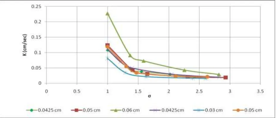
3.1 Variation Of K with σ
To study the effect of non uniformity of sediments on hydraulic conductivity , variation of K has been plotted against standard deviation . Figures 3 shows the variation of K with σ for sample sizes used in this study . From the graph it is clear that as value of σ increases , hydraulic conductivity decreases .
Figure 3 Variation of K with σ 3.2 Comparison of Hydraulic conductivity
Table 7 to 12 shows the comparison of experimental result with empirical models namely Kozeny Carman model, Drag force model , Allen Hazen model and Terzaghi model for each sample used in this study . The comparison of estimated and measured results are shown in the Figures 4 to 9 .
Table 7-Comparison of hydraulic conductivity for sample (1) 0.0425 cm diameter with various models
Expermental (cm/sec)
Kozeny Carman model (cm/sec)
Drag force model (cm/sec)
Allen Hazen model (cm/sec)
Terzaghi model (cm/sec)
Estimated Permeability from Models
Residuals Deviation (%)
637 | P a g e
0.047 0.039 7.39×10⁻³ 0.038 0.022 0.026 0.021 44.68
0.038 0.020 1.35×10⁻³ 0.021 0.013 0.016 0.022 57.89
0.029 3.58×10⁻³ 8.72×10⁻⁹ 3.89×10⁻³ 2.24×10⁻³ 0.0056 0.023 80.68
0.021 4.45×10⁻⁴ 3.45×10⁻¹¹ 5.78×10⁻⁴ 2.96×10⁻⁴ 0.000329 0.021 98.43
Figure
4 Comparison of measured and estimated hydraulic conductivity for sand sample (1) 0.0425 cmdiameter
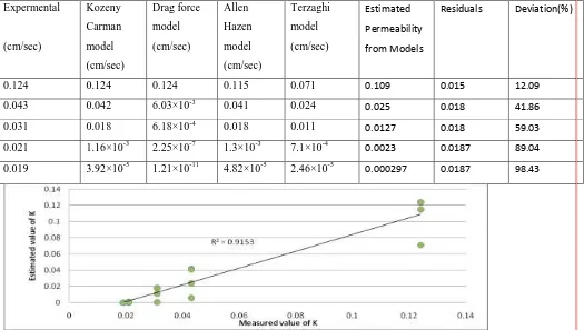
Table 8- Comparison of hydraulic conductivity for sample (2) 0.05 cm diameterwith various models
Expermental
(cm/sec)
Kozeny Carman model (cm/sec)
Drag force model (cm/sec)
Allen Hazen model (cm/sec)
Terzaghi model (cm/sec)
Estimated
Permeability
from Models
Residuals Deviation(%)
0.124 0.124 0.124 0.115 0.071 0.109 0.015 12.09
0.043 0.042 6.03×10⁻³ 0.041 0.024 0.025 0.018 41.86
0.031 0.018 6.18×10⁻⁴ 0.018 0.011 0.0127 0.018 59.03
0.021 1.16×10⁻³ 2.25×10⁻⁷ 1.3×10⁻³ 7.1×10⁻⁴ 0.0023 0.0187 89.04
0.019 3.92×10⁻⁵ 1.21×10⁻¹¹ 4.82×10⁻⁵ 2.46×10⁻⁵ 0.000297 0.0187 98.43
638 | P a g e
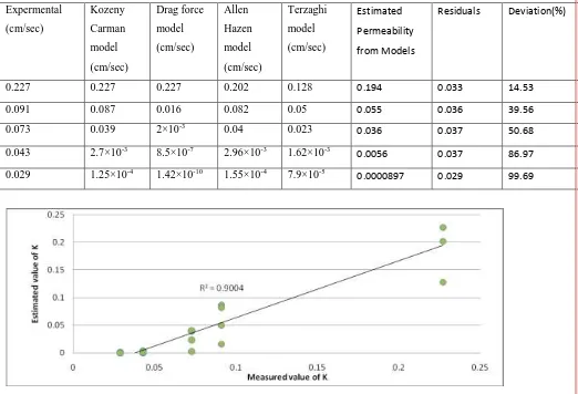
Table 9- Comparison of hydraulic conductivity for sample (3) 0.06 cm diameter with various models
Expermental (cm/sec) Kozeny Carman model (cm/sec) Drag force model (cm/sec) Allen Hazen model (cm/sec) Terzaghi model (cm/sec) Estimated Permeability from Models
Residuals Deviation(%)
0.227 0.227 0.227 0.202 0.128 0.194 0.033 14.53
0.091 0.087 0.016 0.082 0.05 0.055 0.036 39.56
0.073 0.039 2×10⁻³ 0.04 0.023 0.036 0.037 50.68
0.043 2.7×10⁻³ 8.5×10⁻⁷ 2.96×10⁻³ 1.62×10⁻³ 0.0056 0.037 86.97
0.029 1.25×10⁻⁴ 1.42×10⁻¹⁰ 1.55×10⁻⁴ 7.9×10⁻⁵ 0.0000897 0.029 99.69
Figure 6 Comparison of measured and estimated hydraulic conductivity for sand sample (3) 0.06 cm diameter Table 10-Comparison of hydraulic conductivity for sample (4) 0.0425 cm diameter with various models
Expermental (cm/sec) Kozeny Carman Model (cm/sec) Drag force model (cm/sec) Allen Hazen model (cm/sec) Terzaghi model (cm/sec) Estimated Permeability from Models
Residuals Deviation(%)
0.112 0.112 0.112 0.096 0.062 0.093 0.019 16.96
0.07 0.064 0.03 0.058 0.036 0.048 0.022 31.42
0.05 0.034 6.5×10⁻³ 0.034 0.02 0.027 0.023 46
0.03 0.003 6.73×10⁻⁶ 0.003 1.93×10⁻³ 0.0053 0.025 82.33
639 | P a g e
Figure 7 Comparison of measured and estimated hydraulic conductivity for sand sample (4) 0.0425 cm diameter
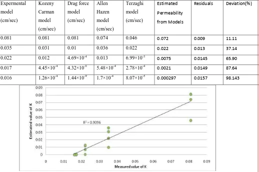
Table 11- Comparison of hydraulic conductivity for sample (5) 0.03 cm diameter with various models
Expermental model (cm/sec)
Kozeny Carman model (cm/sec)
Drag force model (cm/sec)
Allen Hazen model (cm/sec)
Terzaghi model (cm/sec)
Estimated
Permeability
from Models
Residuals Deviation(%)
0.081 0.081 0.081 0.074 0.046 0.072 0.009 11.11
0.035 0.031 0.01 0.036 0.022 0.022 0.013 37.14
0.022 0.012 4.69×10⁻⁴ 0.013 6.99×10⁻³ 0.0075 0.0145 65.90
0.017 4.45×10⁻⁴ 4.32×10⁻⁸ 5.48×10⁻⁴ 2.78×10⁻⁴ 0.0021 0.0149 87.64
0.016 1.26×10⁻⁴ 1.44×10⁻⁹ 1.7×10⁻⁴ 8.07×10⁻⁵ 0.000297 0.0157 98.143
640 | P a g e
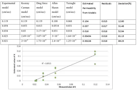
Table 12 Comparison of hydraulic conductivity for sample (6) 0.05 cm diameter with various models
Expermental model (cm/sec)
Kozeny Carman model (cm/sec)
Drag force model (cm/sec)
Allen Hazen model (cm/sec)
Terzaghi model (cm/sec)
Estimated
Permeability
from Models
Residuals Deviation(%)
0.119 0.119 0.119 0.108 0.068 0.104 0.015 12.60
0.054 0.053 0.013 0.0514 0.031 0.037 0.017 31.48
0.034 0.03 3.17×10⁻³ 0.031 0.018 0.016 0.018 52.94
0.023 2.69×10⁻³ 3.07×10⁻⁶ 3×10⁻³ 1.64×10⁻³ 0.00434 0.019 81.13
0.021 2×10⁻⁴ 1.73×10⁻⁹ 2.4×10⁻⁴ 1.25×10⁻⁴ 0.00226 0.019 89.23
Figure 9 Comparison of measured and estimated hydraulic conductivity for sand sample (6) 0.05 cm diameter