Performance Analysis of the Recursive Least
Squares Algorithm
Writi Mitra
1, Subhojit Malik
2Assistant Professor, Department of ECE, Hooghly Engineering and Technology College, Hooghly, West Bengal, India1,2
ABSTRACT: Adaptive filter algorithm is a widely used method in communication systems, control systems, digital signal processing etc. This method helps to find out the unknown parameters iteratively by adjusting the filter parameters. There are many efficient adaptive filter algorithms. But among them, the basic algorithms are: Least Mean Square (LMS) and Recursive Least Square (RLS) Algorithms. The LMS algorithm is based on gradient optimization and the RLS algorithm is based on direct form FIR and lattice realization. The RLS algorithm is popular because of its fast convergence although the LMS algorithm is very simple to implement. There are modified LMS algorithms and they are: Leaky Least Mean Square (LLMS) Algorithm and Normalized Least Mean Square (NLMS) Algorithm. „Step size‟ is an important parameter which is used to implement any of these LMS algorithms. In case of RLS algorithm, one term „forgetting factor‟ plays an important role in times of implementing any system.
KEYWORDS:Recursive Least Square (RLS) Algorithm, Least Mean Square (LMS) Algorithm, Leaky Least Mean Square (LLMS) Algorithm, Normalized Least Mean Square (NLMS) Algorithm, Frequency Response Curve, Coefficient Response Curve, Error Response Curve, Step Size, Forgetting Factor.
I.INTRODUCTION
Adaptive filter is a popular filter which is used in the domain of Digital Signal Processing (DSP). It has received considerable attention from the researchers for last forty years. Naturally good number of efficient adaptive filtering methods has been developed within this span of time. Now, in times of designing an intelligent system, adaptive process is required [7-10]. As a designer, a digital system is always preferable because of its small size, lower cost, fast speed of operations and flexibility in operation. In the field of DSP, adaptive filter algorithm is a popular tool to design any intelligent system. The digital filters may be classified as Infinite Impulse Response (IIR) and Finite Impulse Response (FIR) Filters. FIR filters are preferred for more stable design due to the lack of feedback in the design and such reliable design in will affect the evolution on adaptive process.
An adaptive filter is a filter which is implemented by using error signal with adjustable coefficients. In times of implementing any adaptive process, a cost function is taken for optimization purpose. The optimum solution of the algorithm can be achieved by minimizing the cost function.The adaptive process is time varying and non-linear in nature.
In this paper the basics of RLS and LMS adaptive filtersalgorithms are surveyed and discussed. The Recursive Least Square (RLS) algorithm is surveyed and discussed. At the same time for doing the comparison, the Least Mean Square (LMS) algorithm is also discussed. The LMS algorithm is the basic algorithm which is used for any adaptive filter and the modified LMS algorithms are Normalized Least Mean Square (NLMS) and Leaky Least Mean Square (LLMS) Algorithms which are also discussed very briefly.
In the next section of the paper, the Adaptive Filtering Algorithms (II), the RLS and different LMS algorithms, the implementation of RLS and different LMS Algorithms (III), the Result Analysis (IV), the Conclusion (V) and the References are given.
II.ADAPTIVE FILTERING ALGORITHMS
To design an adaptive filter, adaptive filter algorithm is used iteratively. The basic block diagram of adaptive filter is given in figure (1). For any adaptive process, the error signal ,e(n) which iscalculated as
[ ]
[ ]
[ ]
(1)
wherethe number of iteration is n, the input signal is denoted by x(n), the adaptive-filter output signal is y(n) and d(n) is the desired signal.
Figure1: Basic Adaptive Filter Algorithm Scheme
To form an objective function, the error signal is used. In order to determine the appropriate filtercoefficients, the adaptation algorithm is used. The minimization of objective function will help the adaptive-filter output signal to match with the desired signal. So the error signal is formed and optimized to find the optimized solution. Hence the choice of error signal in an adaptive algorithm is very important. The overall convergence process also influences the adaptive algorithm. A filter consists with many coefficients. There are many methods for performing weight update of an adaptive filter. The different filtering algorithms are: Recursive Least Square (RLS) ,Least Mean Square (LMS), Normalized Least Mean Square (NLMS) and Leaky Least Mean Square (LLMS)[1,9,10].
Recursive Least Squares Algorithm
The Recursive Least Squares(RLS) algorithm is also used to find out the coefficient of adaptive filter. The algorithm uses information from all past input samplesto estimate the autocorrelation matrix of the input vector. To decrease the influence of inputsamples from the past, a weighting factor for the influence of each sample isused. This weighting factor is introduced in the cost function. The cost function is denoted by
2
1
[ ]
[ , ]
(2)
n n i
i
J n
p
e i n
Here, the error signal e[i,n] is computed for 1 ≤ i ≤ n using the current filter coefficients c[n] and the error signal is denoted by
[ , ]
[ ]
H[ ] [ ]
(3)
e i n
d i
c
n x i
The coefficient update equation is given by in equation (10)
[ ]
[
1]
[ ]*{ [ ]
H[ ] [
1]}
(4)
c n
c n
k n
d n
x
n c n
To update the coefficient, the following informations are required.
1
[ ]
[ ]
(5)
p n
n
Here p[n] can be represented by using the update equation (12) with the help of matrix inversion lemma. Now the value of p[n] can be founded by
1
[ ]
[
1]
[ ] [ ]
(6)
p n
p n
k n x n
And the value of k[n] can be calculated by using equation (13)
1
1
[
1] [ ]
[ ]
(7)
1
H[ ] [
1] [ ]
p n
x n
k n
x
n p n
x n
The value λ is also termed as forgetting factor.
Least Mean Square Algorithm
Least Mean Square (LMS) was developed by Windrow & Holf in 1959. The steepest descent approach is usedin LMS algorithm for estimating the gradient vector for deriving a cost function[7-10].Thesample values of the tap-input vector and an error signal are used for estimating the gradient. To check the performance of any algorithm, it is necessary to use a reference signal d[n] and this reference signal is taken as the desired filter output. Thedifference between the reference signal and the actual output is taken as the error signal which is represented in Equation 2.
[ ]
[ ]
H[ ] [ ]
(8)
e n
d n
c
n x n
A set of filter coefficients is represented by c and this set of coefficients is minimizedfor the expected value of the quadratic error signalto achieve the least mean squared error. To update the coefficients in LMS algorithm, Equation 3 is used and it depends on every time instant n,
*
[
1]
[ ]
[ ] [ ]
(9)
c n
c n
e n x n
In this context, the selection of the parameter „step-size‟(µ) in equation 3 is important. The movement of coefficients along the error function surface at each updated step is controlled by varying the step size.
Leaky Least Mean Square Algorithm
In Leaky LMS (LLMS) algorithm, the cost function is defined by the following equation:
1
2 2
0
[ ]
[ ]
[ ]
(10)
N i i
j n
e n
w n
whereγ is the leaky factor and the range of γis 0 to 0.1. The cost function of the LLMS algorithm is different from thestandard LMS algorithm. The leaky LMS algorithm updates thecoefficients of an adaptive filter by using the following equation:
[
1]
(1
) [ ]
[ ] [ ]
(11)
w n
w n
e n u n
Now another term µ is present in leaky LMS. In leaky LMS algorithm, the migration of coefficients may cause an overflow problem.
If γ = 0, the leaky LMS algorithm becomes the same as the standard LMSalgorithm. A steady state error may arise for selecting a large leaky factor is chosen,
Normalized Least Mean Square Algorithm
The simple LMS algorithm is sensitive to the scaling of its input x(n). Due to this reason, it is important to choose a learning rate μ properly. At the same time, the parameter must be chosen in such a way that the stability of the algorithm may not hamper. This problem can be overcome by using the recursion formula of Normalized Least Mean Square (NLMS) algorithm which is stated in equation 12;
[
1]
[ ]
[ ] [ ] [ ]
(12)
w n
w n
n e n u n
Here, µ[n] is the step size and it is varying with the time.
[ ]
(13)
[ ]
T[ ]
n
x n x n
c
µ[n] is denoted by Equation 7 and c is a small positive constant to avoid division by zero and β is normalized step- size nearly varying form 0< β <2.
III. IMPLEMENTATION OF ADAPTIVE FILTER ALGORITHMS
So the Blackman window function is expressed as:
2
4
[ ]
0.42 0.5cos(
) 0.08cos(
)
(14)
1
1
n
n
w n
N
N
where , 0 ≤ n ≤ N-1 The input is taken as
[ ]
sin(
c(
)). /( *(
))
(15)
x n
n alpha
eps
n alpha
eps
wherewc is the cut-off frequency, eps=phase=0.001 and alpha=( No. of taps-1) /2 ;
Finally the RLS, LMS, LLMS and NLMS algorithms are implemented by using MATLAB and the system is tested by using the above input with Blackman window function. A comparative study of system outputs are carried out by fixing all depending parameters of all the algorithms.
IV. RESULT ANALYSIS
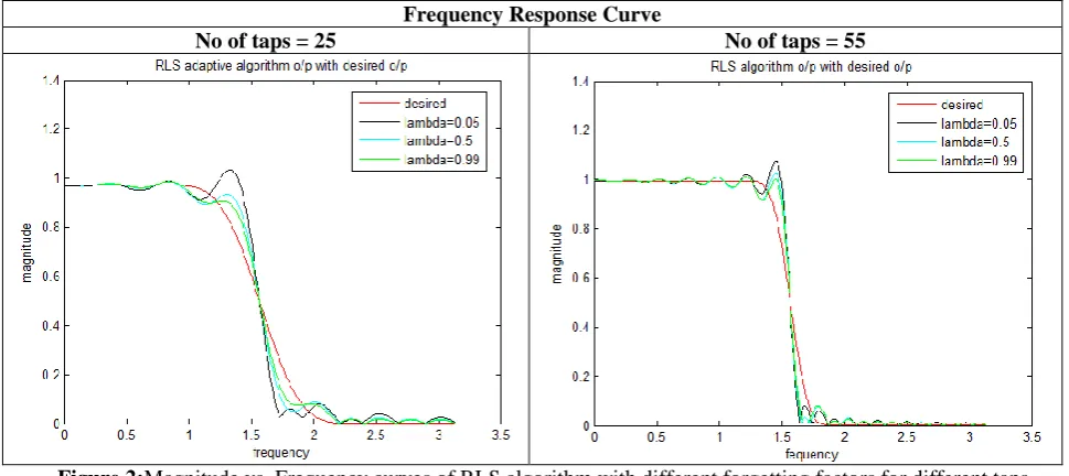
To analyse the RLS algorithm, the test system is a low pass filter (LPF). In times of designing, a finite impulse response (FIR) type LPF is used and that FIR filter is preferred to design by using Blackman window function. Initially the RLS algorithm is applied to find out the frequency response for different values of the forgetting factor (λ). The coefficient response curves and the error response curves are also plotted. Finally the LMS, LLMS and NLMS Algorithms are applied to the system and the frequency response curves for these systems are plotted and compared against the response curve that we have obtained for RLS algorithm. The number of iterations is taken as 1000. The frequency response curves are plotted by varying the number of taps with varying forgetting factors.
Frequency Response Curve
No of taps = 25 No of taps = 55
Figure 3:Coefficient response curves using RLS Algorithm with different forgetting factors
In figure 3, we observe that if the value of λ is increased, the response of the coefficient response becomes best.
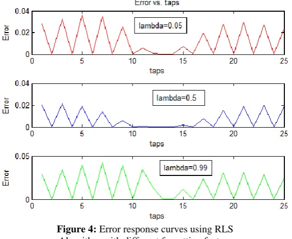
Figure 4: Error response curves using RLS Algorithm with different forgetting factors
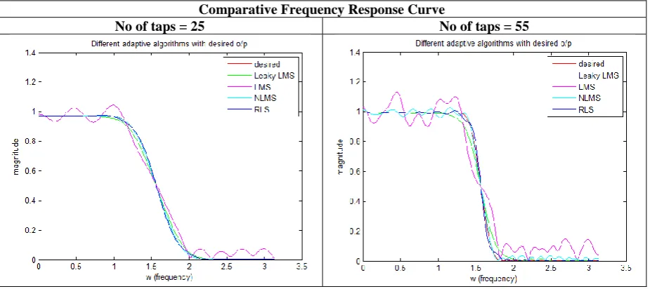
Comparative Frequency Response Curve
No of taps = 25 No of taps = 55
Figure 5: Comparative study on Frequency response curves of adaptive algorithm for different taps
In figure 5, we observe that the frequency responses of LMS, NLMS, LLMS and RLS are plotted together. Now wecan notice thatwe get best response for NLMS when the number of taps is taken as 25. Now considering the number of taps as 55, the responses correspond to LMS, NLMS, LLMS got distorted but the response of RLS get better than response when the number of tap was 25.
So, if the number of tap value is increased, responses ofLMS, NLMS, and LLMS get noisy and RLS get better response. Hence, the RLS algorithm shows a better response with the increase of number of taps.
V.CONCLUSION
In case of RLS algorithm, the range of forgetting factor must be chosen in such a way that we get reduced oscillation. In this paper, we kept the range 0 <λ< 1. We get less oscillation when λ=0.5 in the frequency response curve. At the same time the amount of error is less when the forgetting factor is chosen as λ =0.5 in the error response curve. If the value of λ is increased, the better coefficient response can be obtained.
If the number of iterations and the step size of all adaptive algorithms are kept constant, the responses ofLMS, NLMS, and LLMS get noisy but the response of RLS algorithm get better with the increased step size. Hence, the RLS algorithm shows a better response with the increase of number of taps.
REFERENCES
[1] Syed AteequrRehman, R.Ranjith Kumar, “Performance Comparison of Adaptive Filter Algorithms for ECG Signal Enhancement”, International Journal of Advanced Research in Computer and Communication Engineering Vol. 1, Issue 2, April 2012.
[2] Ahmed Elhossini, ShawkiAreibi, Robert Dony, “An FPGA Implementation of the LMS Adaptive Filter for Audio Processing”, IEEE International Conference on Reconfigurable Computing and FPGA's, ReConFig 2006
[3] Asit Kumar Subudhi, BiswajitMishra ,Mihir Narayan Mohanty, “VLSI Design and Implementation for Adaptive Filter using LMS Algorithm”,International Journal of Computer & Communication Technology (IJCCT), Volume-2, Issue-VI, 2011.
[4] “Modified Adaptive Filtering Algorithm for Noise Cancellation in Speech Signals”,V. R. Vijaykumar, P. T. Vanathi,P. Kanagasapabathy, Electronics and Electrical Engineering. – Kaunas: Technologija, 2007. – No. 2(74). – P. 17–20.
[5] J. Malarmannan, S. Malarvizhi, “FPGA Implementation of Adaptive Filter and its Performance Analysis”,International Journal of Engineering and Technology,Vol 5 No 3 Jun-Jul 2013, ISSN : 0975-4024.
[6] Gunnar Tufte and Pauline C. Haddow, Evolving an Adaptive Digital Filter, IEEE transaction, 2000 [7] S.Haykin, Adaptive Filter Theory, Prentice-Hall, 2002.
[8] Dr. Shaila D. Apte, Digital Signal Processing, 2nd Edition, Wiley Publication , 2014
[9] John G. Proakis, Dimitris G. Manolakis, Digital Signal Processing Principles, Algorithms and Applications, Fourth Edition, PHI Publication, 2006.
BIOGRAPHY
Prof. Writi Mitra is an Assistant Professor in the Department of Electronics & Communication Engineering, Hooghly Engineering & Technology College. She has a Master Degree in Digital Systems & Instrumentation from IIEST,Shibpur,India and areas of interest are VLSI Design, Digital Signal Processing and Image Processing.