Assessing time series reversibility through permutation patterns

(1)

Assessing time series reversibility through

permutation patterns

Massimiliano Zanin1,2,∗, Alejandro Rodríguez González1, Ernestina Menasalvas Ruiz1and David Papo3

1 _{Center for Biomedical Technology, Universidad Politécnica de Madrid, 28223 Pozuelo de Alarcón, Madrid,}

Spain.

2 _{Department of Computer Science, Faculty of Science and Technology, Universidade Nova de Lisboa,}

2829-516 Lisboa, Portugal.

3 _{University of Lille, 59800 Villeneuve d’Ascq, France.}

* Correspondence: [email protected]; Tel.: +34-91-336-4632

Version August 4, 2018 submitted to

Abstract: Time irreversibility,i.e. the lack of invariance of the statistical properties of a system 1

under time reversal, is a fundamental property of all systems operating out of equilibrium. Time 2

reversal symmetry is associated with important statistical and physical properties and is related to the 3

predictability of the system generating the time series. Over the past fifteen years, various methods 4

to quantify time irreversibility in time series have been proposed, but these can be computationally 5

expensive. Here we propose a new method, based on permutation entropy, which is essentially 6

parameter-free, temporally local, yields straightforward statistical tests, and has fast convergence 7

properties. We apply this method to the study of financial time series, showing that stocks and indices 8

present a rich irreversibility dynamics. We illustrate the comparative methodological advantages of 9

our method with respect to a recently proposed method based on visibility graphs, and discuss the 10

implications of our results for financial data analysis and interpretation. 11

Keywords:Time irreversibility; permutation entropy; visibility graphs; efficient market hypothesis. 12

1. Introduction 13

Time irreversibility is the lack of invariance of the statistical properties of a signal under the 14

operation of time reversal. In other words, consider a time series describing the evolution of a system, 15

x(t)witht∈ [0,T]and its time reversal,i.e. the time series that would have been obtained had the 16

system evolved in the opposite direction, orxt.r.(t) =x(T−t). Irreversibility means that it is possible 17

to find a characteristic that differs in the forward and backward versions, i.e. a functionf calculated 18

over the two time series such that f(xt.r.₎₆₌ _f₍_x₎_{; or, in other words, that the observer can distinguish} 19

the forward, from the backward version of a given process. Note that the above definition does not 20

impose any restriction onf. 21

Irreversibility can be due to the presence of memory, which acts as a hidden dissipative external 22

force in a process [1] while the presence of noise results in a loss of irreversibility [2]. Thus, estimating 23

the degree of irreversibility of a time series implicitly quantifies the degree of nonlinear dependences 24

(memory), and therefore, the degree of time series predictability. Importantly, since linear Gaussian 25

random processes and static nonlinear transformations of such processes are reversible, significant time 26

irreversibility excludes Gaussian linear processes as models for the generating dynamics, implying 27

instead nonlinear dynamics, non-Gaussian (linear or nonlinear), or linear ARMA models as possible 28

generative processes [3–5]. 29

The mere statistics of observed time series allows extracting information on the physics of the 30

system under study. In particular, time reversal asymmetry provides information about the entropy 31

production of the physical mechanism generating the series, even when the details of the underlying 32

generating system are unknown [6]. Various methods to quantify time reversibility have been proposed 33

and applied to the study of both biological and financial systems [2,7–14]. 34

(2)

Here, we introduce a new method, based on permutation entropy [15,16] to evaluate irreversibility 35

of time series at various temporal scales. With respect to existing methods, the proposed one 36

presents various advantages: 1) it has no free parameters other than the embedding dimension 37

of the permutation entropy; 2) as visibility graph methods [13] it is temporally local, and therefore 38

allows assessing fluctuations; 3) assessing significance is straightforward, and does not rely on scaling 39

arguments as visibility graph methods, over which it also has 4) a convergence speed advantage. 40

We first illustrate our method by evaluating the time irreversibility of a set of simple dynamical 41

models, including stochastic models and chaotic dynamical systems, for which such property has 42

theoretically been studied. We further show how the proposed approach can help elucidating the 43

complex irreversibility dynamics of financial time series, representing 30 major European stocks and 44

12 world indices. 45

The time-reversal properties of financial time series allow testing the so-called efficient market 46

hypothesis (EMH) [11]. The EMH asserts that financial markets are efficient with respect to an 47

information set,i.e. that stocks incorporate all publicly available information useful in evaluating 48

their prices and no single market agent can consistently outperform the market can be made from 49

information based trading [17]. Importantly, efficiency is related to the amount of information available 50

to predict future market prices, with lower efficiency corresponding to higher residual predictive 51

information in the past sequence of stock prices [18]. The stringency of EMH’s requirements suggests 52

that no real market can ever be efficient stricto sensu [19] and that EMH should not be approached 53

as an all-or-nothing property [20]. Various empirical studies have then undertaken to quantify the 54

extent to which the EMH holds and, as a result to identify the sort of process governing market 55

behaviour [20–23]. While financial series have been found to generally be time irreversible [2,7,11,24], 56

it is possible to discriminate different degrees of such property. For instance, some stocks have been 57

found to be more irreversible than others [14]. Likewise, emerging markets have been shown to be 58

more time irreversible than developed ones, lending support to the relationship between efficiency 59

and irreversibility [25]. 60

We show that stocks’ and indices’ time series present a rich dynamics in terms of irreversibility. 61

Specifically, while some time series may globally be reversible, they can become irreversible at 62

specific temporal resolutions,i.e. when windows of specific length are considered. Additionally, 63

such irreversibility may appear in a temporal localised way, suggesting that the dynamics of the 64

element was somehow perturbed at that time. 65

The remainder of the paper is organised as follows. Firstly, the proposed method is described 66

in Section2; we also include a brief overview of the visibility graph (Section2.3) and of the Markov 67

chain (Section2.4) approaches, as they will be used to benchmark our solution. We then validate 68

the permutation patterns’ method in synthetic (Section3) and financial (Section4) time series. Some 69

conclusions are finally drawn in Section5. 70

2. Assessing time series reversibility 71

2.1. Permutation patterns 72

The idea of analysing the permutation patterns present in a time series was initially introduced 73

by Bandt and Pompe [15] to provide researchers with a simple and efficient tool to characterise the 74

complexity of the dynamics of real systems. With respect to other approaches, as entropies, fractal 75

dimensions, or Lyapunov exponents, it presents the advantage of being independent from any arbitrary 76

thresholds or binning procedures [16]. For the sake of completeness, we here briefly review the process 77

of calculating these permutation patterns. 78

Given a time seriesX={xt}, witht=1 . . .N, this is usually divided in overlapping regions of

79

lengthD, such that: 80

(3)

Dis called theembedding dimension, and controls the quantity of information included in each 81

region, whileτis the embedding delay.sfurther controls the beginning of each region, and thus the

82

degree of overlap between regions. Without loss of generality, in what follows we will considerD=3 83

andτ=1.

84

The second step involves associating an ordinal pattern to each region. Values are sorted in 85

increasing order, and the ordinal pattern corresponding to the required permutation is saved for 86

further analysis. In other words, the permutationπ= (r0,r1, . . . ,rD−1)of(0, 1, . . . ,D−1)is defined 87

to fulfil: 88

xs+r0 ≤xs+r1 ≤. . .≤xs+rD−2 ≤xs+rD−1. (2)

To illustrate, suppose a time seriesX= (3, 2, 6, 4, 8). AsD= 3, the first region would include 89

the values(3, 2, 6), and the order required for sorting them is(1, 0, 2)- that is, the second value is the 90

smallest, followed by the first and by the last. Similarly, the second region(2, 6, 4)is associated with 91

the pattern(0, 2, 1); and the third region(6, 4, 8)with(1, 0, 2). 92

2.2. Time reversibility of permutation patterns 93

After estimating all the permutation patterns in a time series, we analyse their frequency of 94

appearance, taking into account a time reversal process. 95

The total number of permutation patterns that may appear is given byD!. These patterns can be 96

paired together, such that each pattern composing a pair is the time reversal of the other. For instance, 97

forD=3, six patterns are generated, which can pairwise be related as: 98

(0, 1, 2)t.r.↔(2, 1, 0) (3)

(1, 0, 2)t.r.↔(2, 0, 1) (4)

(1, 2, 0)t.r.↔(0, 2, 1), (5)

witht.r.↔representing a time reversal transformation. 99

In order to clarify this idea, let us consider the simple example of a time series resembling a 100

sawtooth,X= (1, 2, 3, 1, 2, 3, 1). The series is stationary, as the average oscillates around 2.0, and five 101

permutation patterns of sideD=3 can be extracted:(0, 1, 2),(1, 2, 0),(2, 0, 1),(0, 1, 2)and(1, 2, 0). It 102

can be observed that the system has a non-trivial dynamics, as it always increments in two consecutive 103

steps at the time - hence the upward pattern(0, 1, 2). Let us now consider the time reversed series, 104

i.e. the same series observed from the end to the beginning: X = (1, 3, 2, 1, 3, 2, 1). The new (time 105

reversed) permutation patterns are(0, 2, 1),(2, 1, 0),(1, 0, 2),(0, 2, 1)and(2, 1, 0). As it should be 106

expected, the new time series can only diminish through the(2, 1, 0)permutation pattern - which is, of 107

course, the time reversal equivalent of(0, 1, 2). Note that this allows us to conclude that the time series 108

Xis irreversible: if two consecutive increasing (respectively, decreasing) values are found, then we 109

can conclude that we are observing the direct (time reversed) time series, and we thus have a way of 110

defining a time directionality. This can further be generalised: a time series will be reversible if and 111

only if all permutation patterns composing the previous pairs appear with approximatively the same 112

frequency. This hypothesis will constitute the basis of the reversibility statistical test described below. 113

The value ofD=3 has here been chosen for the sake of clarity. While in principle larger values of 114

Dmay yield a richer description of the dynamics, this also results in the need of longer time series to 115

reach statistically significant results - both topics will be further discussed in the conclusions. 116

The previously defined pattern pairs and their frequency of appearance can be analysed in two 117

ways: in terms of the magnitude of the irreversibility, through the Kullback-Leibler divergence, and in 118

(4)

The irreversibility magnitude can be quantified by comparing two probability distributions, 120

one represented by the probability of all patterns appearing in the direct (or original) time series, 121

and a second one with the probabilities for the time-reversed time series. Following the previous 122

example for D = 3, the first distribution is composed of the frequencies of patterns Pd =

123

[p(0,1,2),p(2,1,0),p(1,0,2),p(2,0,1),p(1,2,0),p(0,2,1)]. As for the second distribution, it can be calculated by 124

actually reversing the time series, or more simply by using the previous time reversal transformations -125

i.e.by considering the distributionPr = [p(2,1,0),p(0,1,2),p(2,0,1),p(1,0,2),p(0,2,1),p(1,2,0)]. The difference 126

between both distributions can then be estimated through the Kullback-Leibler divergence: 127

DKL= D!

∑

i=1

P_d(i)logPd(i)

Pr(i). (6)

If the time series is perfectly reversible, the probabilities associated to patterns forming a pair 128

should be the same, thus yielding aDKL ≈0. On the other hand, the higher the value ofDKL, the

129

more irreversible the time series is. Note thatDKLis not the only possibility for comparing the two

130

distributions, being the Jensen-Shannon divergence a good alternative. While the latter presents the 131

advantage of being symmetric, the former is commonly used in statistical physics [13,26]. Additionally, 132

it has to be noted that Eq.6diverges when one or more permutation patterns are forbidden,i.e.their 133

frequency is zero. This may happen when the time series under analysis is trivially irreversible (and 134

possibly non-stationary), as is the case of a ramp function. This can easily be solved by adding a very 135

small value to all probabilities,i.e. 136

DKL= D!

∑

i=1

Pd(i)log

Pd(i) +e

Pr(i) +e, (7)

such thateminPdandeminPr. This situation is nevertheless seldom encountered in real

137

time series, provided their length is large enough. 138

If the Kullback-Leibler divergence tells us the magnitude of the irreversibility of a time series, it 139

yields little information about the statistical significance of the value. This problem can be solved by 140

levering on the binomial nature of the patterns composing a pair. Specifically, if the time series 141

is reversible, the number of times the two permutation patterns forming a pair appear should 142

not statistically be different. Following the previous example, let us denote byn(0,1,2)andn(2,1,0) 143

respectively the number of times the patterns(0, 1, 2)and(2, 1, 0)have appeared; and let us define: 144

p= n(0,1,2) n(0,1,2)+n(2,1,0)

. (8)

The time series is not reversible if we can reject the null hypothesis thatp=0.5 in a two-sided 145

binomial test. Note that the test should be repeated for all pairs of permutation patterns - three times 146

in the case ofD=3. 147

One final discussion should here be added on the relationship between irreversibility and 148

stationarity, and how such relationship affects the proposed methodology. On one hand, it is intuitive 149

that a non-stationary process must also be irreversible - as a net change from stateato statebnecessarily 150

implies a time direction. Time irreversibility has therefore normally been assessed only in the presence 151

of stationarity. On the other hand, it has recently been proposed that reversibility can be assessed even 152

in non-stationary systems, by moving from a qualitative to a quantitative metric [26]. In the case of 153

the methodology here proposed, the degree of irreversibility of a time series can be assessed by the 154

magnitude ofDKL(or of a Jensen-Shannon divergence), provided no permutation pattern is forbidden,

155

i.e.Pr(i)>0 for alli. This quantitative aspect will be further explored in Section4.

(5)

2.3. Directed Horizontal Visibility Graphs 157

One of the most recent and efficient ways of assessing the irreversibility of a time series is through 158

the so-called directed Horizontal Visibility Graphs (dHVG). In what follows, this method is used for 159

benchmark purposes, and, for the sake of completeness, is here briefly introduced. 160

From a general point of view, dHVG belong to a family of methods that map a time series into 161

nodes of a network, based on geometric criteria [27,28]. In all of these methods, a complex network 162

[29] is created, whose nodes correspond to the individual data of the time series; pairs of nodes are 163

then connected when they fulfil some geometrical rule, usually based on whether one value can “see” 164

the other one. In the specific case of dHVG, two nodes are connected if the line connecting both values 165

is not obstructed by another intermediate point [28]. Mathematically, given two nodesiandj, a link is 166

created if: 167

xi,xj>xn,∀n|i<n<j, (9)

beingxithe element of the time series mapped into nodei.

168

The resulting network can then be analysed using the wide set of tools provided by complex 169

networks theory [30]. Of relevance for this work, the irreversibility of a time series can be assessed by 170

comparing the distributions of in- and out-degrees (i.e.respectively the number of links arriving to 171

and departing from a given node), and by calculating a Kullback-Leibler divergence [13,14]. Note that 172

the in-degree of a node becomes its out-degree under a time reversal transformation. Therefore, for 173

reversibility to holds both distributions ought to be equal, and the corresponding Kullback-Leibler 174

divergence should converge to zero. For more details on the dHVG approach and the assessment of 175

irreversibility, we refer the reader to the following studies [13,14,28]. 176

2.4. Markov chain approach 177

We finally consider a classical method for detecting time series irreversibility, based on the 178

representation of the underlying system as a Markov chain. In the case of a Markov chain with a 179

transition matrixPi,jand steady-state distributionsπi, time symmetry impliesπiPi,j=πjPj,i; a time

180

series is then reversible if and only ifPi,j = Pj,i, for allis and j 6= i [31]. We use this property to

181

construct a simple test, which requires:i) binning the elements of the original time series into a set 182

of bins (note that the number of bins is a parameter of the method);ii) calculate the transition matrix 183

Pi,j; andiii) perform a binomial statistical test on each pair(i,j), withj6=i, to test the hypothesis that

184

Pi,j=Pj,i.

185

3. Validation with synthetic time series 186

We validate the permutation patterns approach to irreversibility assessment, and compare it with 187

the visibility graph one, through the application to a set of synthetic time series whose reversible or 188

irreversible nature has already been studied theoretically. These are: 189

• Two reversible stochastic processes, namely a time series of values drawn from a Gaussian 190

distributionN(0, 1), and an Ornstein-Uhlenbeck process, a mean-reverting linear Gaussian 191

process T[32]. 192

• Two dissipative chaotic maps, respectively a logistic map (defined asxn+1=axn(1−xn), with

193

a = 4.0) and a Henon map (xn+1 = 1+yn−ax2t, yn+1 = bxt, with a = 1.4 andb = 0.3).

194

Dissipative systems are by definition irreversible [33]. 195

• The Arnold Cat map, and example of a conservative chaotic map (xn+1 = xn +yn

196

mod (1),yn+1 = xn+2yn mod (1). The analysed time series corresponds to the evolution

197

of thexvariable. 198

• The Lorenz chaotic system, defined as ˙x = σ(y−x), ˙y = x(ρ−z)−y, and ˙z= xy−βz(with

199

ρ=28,σ=10 andβ=8/3, integration step ofdt=0.01). Unless otherwise stated, the analysed

200

(6)

101 ₁₀2 ₁₀3

Time series length

10-4 10-3 10-2 10-1 100

<

D

>

>

Lorenz system

Irreversibility

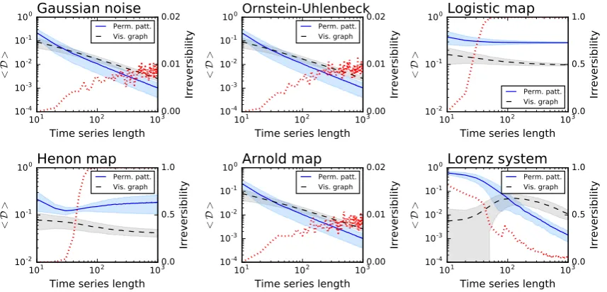
Figure 1.Irreversibility analysis of several synthetic dynamical models, as a function of the time series length. From left to right, top to bottom, the six panels represent Gaussian noise, an Ornstein-Uhlenbeck process, logistic, Henon and Arnold maps, and a Lorenz oscillator - see main text for details and parameters. In the left Y axis, the blue solid and black dashed lines respectively represent the average KullbackLeibler divergence obtained by the permutation patterns and the visibility graph approach -note the blue and grey bands, depicting one standard deviation. On the right Y axis, the dotted red line indicates the fraction of simulations in which the time series is irreversible in a statistical significant way, withα=0.01.

For each of them, Fig.1reports:i) the average divergenceDyielded by the permutation patterns 202

(blue line and one standard deviation band) and the visibility graph (black line and band) approaches; 203

andii) the fraction of times the time series is detected as irreversible by the permutation patterns 204

approach in a statistical significant way (red dotted line, right Y axis, significanceα=0.01). The two

205

examples of stochastic processes and the Arnold map are recognised as irreversible in less than 1% 206

of the realisations - as expected from the choice of a statistical significance level ofα=0.01. On the

207

other hand, the irreversibility frequency rapidly converges to one for the two dissipative chaotic maps 208

- which are known to be irreversible [33]. Finally, a special situation can be observed for the Lorenz 209

system: while its time series are mostly irreversible at short temporal scales, they become highly 210

reversible when sufficiently long time windows are considered. To understand if such behaviour is a 211

general property of the system, Fig.2Left reports the evolution of the irreversibility as a function of 212

time series length, for the three channels of the Lorenz system. While theXandYchannels have a 213

similar dynamics, theZone is substantially different: first it is completely irreversible over long time 214

scales, and second, the evolution of the irreversibility is not monotonic, with a minimum around 70 215

and a peak every 60 time points. This abnormal behaviour for theZtime series is possibly due to its 216

dynamics, which is well known to differ from those of theXandYchannels in terms of Lyapunov 217

exponent [34] and autocorrelation (see Fig.2Right). 218

Fig. 1further suggests that the permutation patterns approach to irreversibility can be more 219

sensitive than the visibility graph one - note that the<D>blue lines usually have a steeper slope, and 220

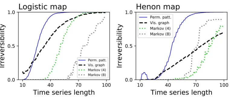
converge faster than the black ones. Fig.3depicts the fraction of times the three considered methods 221

detect that the underlying time series is irreversible in a statistical significant way (α=0.01), for very

222

short time series lengths and for the two systems that were detected as irreversible (i.e.respectively 223

the Logistic and the Henon maps). Note that, in order to calculate the statistical significance of the 224

(7)

10

1

₁₀

2

₁₀

3

Time series length

0.0

0.2

0.4

0.6

0.8

1.0 Irreversibility

Lorenz system

X

Y

Z

0

100

200

300 Lag

0.4

0.0

0.4

0.8 Auto-correlation

X

Y

Z

Figure 2.(Left) Fraction of irreversible time series yielded by a Lorenz chaotic system, as a function of the time series length. Black (dashed), blue (solid) and red (dash-dot) lines correspond respectively to theX,YandZchannels of the system. (Right) Autocorrelation of the same three time series.

10

40

70

100 Time series length

0.0

0.5

1.0 Irreversibility

Logistic map

Perm. patt. Vis. graph Markov (4) Markov (8)

10

40

70

100 Time series length

0.0

0.5

1.0 Irreversibility

Henon map

Perm. patt. Vis. graph Markov (4) Markov (8)

Figure 3.Analysis of the time series length required to reach a consistent irreversibility assessment. Both panels depict the fraction of times the permutation patterns (blue solid lines), the visibility graph algorithms (black dashed lines) and the Markov chain method (dotted lines) detect a statistically significant irreversibility, as a function of the time series length. Left and right panels respectively correspond to the logistic and Henon maps.

from randomly shuffled versions of the time series, and the probability of finding a largerDin the 226

random realisations expressed as ap-value. Fig.3indicates that the permutation pattern approach 227

requires shorter time series to reach a consistent output, something that is particularly conspicuous in 228

the case of the Henon map. Additionally, these results highlight the benefit associated to parameter-free 229

methods. Specifically, the Markov chain method has been tested with two different numbers of bins, 230

respectively 4 (green dotted lines) and 8 (grey dotted lines), yielding different results depending on 231

the underlying dynamics. The fact that the proposed methodology required no parameter estimation 232

or tuning thus becomes an important practical advantage. 233

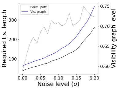
Finally, Fig.4explores the resilience of the proposed method with respect to the presence of noise. 234

Specifically, we consider the previously described logistic map, and added a Gaussian noise: 235

(8)

0.00

0.05

0.10

0.15

0.20 Noise level ( )

100

200

300 Required t.s. length

Perm. patt. Vis. graph

0.60

0.65

0.70

0.75 Visibility graph level

Figure 4.Resilience to noise. The two solid lines (left Y axis) depict the evolution of the time series length required to reach a 90% detection of irreversibility for the logistic map, according to the permutation patterns approach (black) and the visibility graph one (blue), as a function of the level noise. The dashed line (right Y axis) indicates the fraction of times the visibility graph method is detecting an irreversibility, when the permutation patterns method has reached a 90%.

witha= 4.0 andξbeing independent random numbers drawn from a Gaussian distribution

236

N(0, 1). Note that noise is inherently reversible, and therefore its presence is expected to mask the 237

irreversibility of the logistic map. We then measure the minimum time series length that allows to 238

detect the irreversibility of the system the 90% of the times, and plot this as a function of the noise level 239

σ. The two solid lines in Fig.4report the results, and indicate that the permutation patterns approach

240

is more resilient than the visibility graph one. 241

Taken together, the numerical experiments carried out on synthetic time series indicate that the 242

permutation patterns approach is comparable to the visibility graph one in assessing irreversibility. 243

The former is nevertheless more sensitive, as it relies more on local patterns (of dimensionD), and 244

more resilient to noise, thus more suitable for the analysis of short time series. We will take advantage 245

of this in Section4, by analysing the temporal evolution of the irreversibility of real time series. Finally, 246

the local nature of the permutation patterns approach makes it extremely computationally efficient 247

- with a computational cost that scales linearly with the number of data points, as opposed to the 248

quadratic growth of the visibility graph approach. 249

4. Application to financial time series 250

In order to further validate the proposed methodology, we assess the irreversibility of several 251

financial time series. These can be thought of as relatively short realisations of complex stochastic 252

processes whose dynamics is richer than most of the generated time series, and their characteristics 253

(including reversibility) can change over time. Dynamical repertoire richness and time series shortness 254

are two desirable aspects from a validation view-point. As previously introduced, if financial time 255

series were shown to be irreversible, i.e. if some permutation patterns were favoured over their 256

corresponding time-reversed counterparts, this would disprove the efficient market hypothesis (EMH) 257

[11], as the asymmetry would be associated with information with which to improve the prediction of 258

future prices. 259

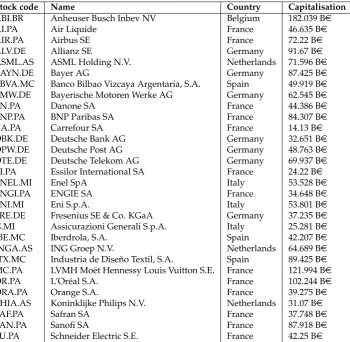
We consider two sets of time series representing the daily evolution of, on one hand, the top-30 260

European stocks by capitalisation; and, on the other hand, of 12 representative world stock market 261

indices. Tabs.1and2report the two full lists, along with some basic characteristics. Both sets of time 262

series have been obtained through Yahoo Finance, and include data from January 1st2008 to January 263

1st2018 - note that the actual number of data points may differ,e.g. due to local bank holidays. In 264

order to ensure the stationarity of all time series, the original valuesXthave been transformed to

265 ˆ

Xt=log₂Xt+1/Xt. The resulting series ˆXhave been tested through an Augmented Dickey-Fuller unit

(9)

Table 1.List of the 30 considered stocks.

Stock code Name Country Capitalisation

ABI.BR Anheuser Busch Inbev NV Belgium 182.039 Be

AI.PA Air Liquide France 46.635 Be

AIR.PA Airbus SE France 72.22 Be

ALV.DE Allianz SE Germany 91.67 Be

ASML.AS ASML Holding N.V. Netherlands 71.596 Be

BAYN.DE Bayer AG Germany 87.425 Be

BBVA.MC Banco Bilbao Vizcaya Argentaria, S.A. Spain 49.919 Be

BMW.DE Bayerische Motoren Werke AG Germany 62.545 Be

BN.PA Danone SA France 44.386 Be

BNP.PA BNP Paribas SA France 84.307 Be

CA.PA Carrefour SA France 14.13 Be

DBK.DE Deutsche Bank AG Germany 32.651 Be

DPW.DE Deutsche Post AG Germany 48.763 Be

DTE.DE Deutsche Telekom AG Germany 69.937 Be

EI.PA Essilor International SA France 24.22 Be

ENEL.MI Enel SpA Italy 53.528 Be

ENGI.PA ENGIE SA France 34.648 Be

ENI.MI Eni S.p.A. Italy 53.801 Be

FRE.DE Fresenius SE & Co. KGaA Germany 37.235 Be

G.MI Assicurazioni Generali S.p.A. Italy 25.281 Be

IBE.MC Iberdrola, S.A. Spain 42.207 Be

INGA.AS ING Groep N.V. Netherlands 64.689 Be

ITX.MC Industria de Diseño Textil, S.A. Spain 89.425 Be

MC.PA LVMH Moët Hennessy Louis Vuitton S.E. France 121.994 Be

OR.PA L’Oréal S.A. France 102.244 Be

ORA.PA Orange S.A. France 39.275 Be

PHIA.AS Koninklijke Philips N.V. Netherlands 31.07 Be

SAF.PA Safran SA France 37.748 Be

SAN.PA Sanofi SA France 87.918 Be

SU.PA Schneider Electric S.E. France 42.25 Be

Table 2.List of the 12 considered market indices.

Index code Name Country

BVSP IBOVESPA Brasil

DJI Dow Jones Industrial Average USA

FCHI CAC 40 France

GDAXI DAX Germany

GSPC S&P 500 USA

HSI Hang Seng Index Hong Kong

IXIC NASDAQ Composite USA

MERV MERVAL Buenos Aires Argentina

MXX IPC Mexico Mexico

N100 EURONEXT 100 Europe

N225 Nikkei 225 Japan

STOXX50E EURO STOXX 50 Europe

root test [35], and for all of them the presence of a unit root was rejected in a statistically significant 267

way (the largerp-value being 2.48·10−14_{for the BNP.PA stock).} 268

Each time series was analysed in three different ways. The first one entails estimating global 269

irreversibility,i.e.taking into account the whole time series. This corresponds to the irreversibility of 270

the system, under the assumption that such property is stationary, or to the assessment of the average 271

irreversibility. Three stocks and four indices resulted irreversible: respectively BBVA.MC, ENEL.MI, 272

G.MI, and DJI, GDAXI, GSPC and IXIC. This indicates that markets have preferred ways (or patterns) 273

when rallying up- or downwards, and are therefore strictly not efficient. It is also interesting to observe 274

(10)

suggest that irreversibility is a collective (or emergent) phenomenon, which is difficult to see in the 276

dynamics of individual elements, but shows up when considering groups of them. 277

Even when the complete time series is reversible, it is possible to find shorter sub-windows 278

which are not reversible in a statistically significant way. Thus, it may happen that time series are 279

globally reversible, but locally irreversible. We explore this possibility in a second analysis, in which 280

we extract all possible sub-windows of a given length from each time series, and calculate their average 281

irreversibility. Note that this allows estimating irreversibility as a function of the time window length, 282

and thus the relationship between irreversibility and time scales. In other words, this second approach 283

enables to study the localvs.global nature of irreversibility. Results of this analysis, in terms of the 284

fraction of windows yielding a statistically significant irreversibility (α=0.01) as a function of the

285

window length, are presented in Figs.5and6. Three general patterns can be distinguished. First of 286

all, many time series that are globally reversible display noisy results, with very low irreversibility 287

probabilities, and usually around or below the significance threshold. Secondly, those time series that 288

are globally irreversible gain such properties at relatively long time scales - the evolution of the fraction 289

of irreversible windows constantly increases with the window size. Finally, some time series, which 290

are globally reversible, can contain irreversible windows with a significant probability; it thus seem 291

that, for those time series, irreversibility is a property confined to some specific time scales. This is the 292

case, for instance, of BAYN.DE (maximum of 20.12% for lengths of 225) or CA.PA (13.89% at 575). 293

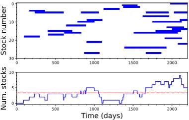
Given that irreversibility is, in many cases, a localised effect, we finally checked whether different 294

stocks present a synchronised dynamics;i.e.if different stocks tend to become irreversible at the same 295

time. Fig. 7presents a time map of the irreversibility of the 30 analysed stocks, when considering 296

windows of 200 data points. While irreversibility seems to be slightly more probable at the end of the 297

considered period, deviations from the expected value are not enough to support the hypothesis of a 298

synchronous dynamics. 299

5. Discussion and conclusion 300

We proposed a new method to quantify irreversibility in time series based on permutation entropy. 301

We tested our method on synthetic time series from various processes with known irreversibility 302

properties and on financial time series of stock prices and indices. For synthetic time series, the results 303

from our method are consistent with known irreversibility properties of the respective time series. 304

Remarkably, particularly for the Lorenz system, the method could detect non-trivial irreversibility 305

dynamics. Our results also show that while most financial time series are globally reversible, the 306

proposed method highlighted an interesting dynamics, with time windows in which the dynamics 307

was significantly irreversible. While the results from the permutation entropy-base method were in 308

line with those obtained with the dHVG-based method, see Fig. 8, the former method compared 309

favourably in terms of convergence speed, indicating that it can be more suitable for relatively short 310

time series. Additionally, the proposed method is able to better handle singular situations, provided 311

the modified version of Eq.7is used. For instance, it is able to detect the extreme irreversibility of a 312

ramp function; on the contrary, for such time series the dHVG-based method yields regular networks 313

with a constant degree of 1, as in both directions each value can only “see” the following one, thus 314

returning aDof zero and wrongly suggesting a perfect reversibility. 315

Our results with synthetic time series are consistent with theoretical results, indicating that the 316

proposed method correctly identifies the underlying process. On the other hand, some results for 317

financial time series are somehow surprising. In particular, our method returned higher irreversibility 318

for some markets previously known to be among the most efficient ones (see Fig.6). These results 319

were in good agreement with those obtained using dHVGs. Insofar as the presence of irreversibility 320

has been associated with violation of the EMH, our results suggest that permutation entropy-based 321

irreversibility and dHVGs may capture a dynamical feature that differs from standard measures of 322

market efficiency. Further investigations will need to clarify the reasons for this discrepancy as well as 323

(11)

0 500 1000 0.00

0.03 0.06

ABI.BR

0 500 1000

0.000 0.025 0.050

AI.PA

0 500 1000

0.000 0.025 0.050

AIR.PA

0 500 1000

0.000 0.004 0.008 0.012

ALV.DE

0 500 1000

0.000 0.008

0.016

0 500 1000

0.000 0.015

Figure 5. Reversibility of the 30 biggest European stocks by capitalization. The solid line of each panel depicts the fraction of windows in which the absence of reversibility was statistically significant (α=0.01), as a function of the window size. The horizontal dashed line represents the significance level of 0.01. An asterisk in the top right corner of a panel indicates that the stock is reversible when considering the whole time series.

One final note should be made on the choice of the embedding dimensionD, which we set to 325

D=3 in this study. Using higher values ofDincreases the richness with which the dynamics of the 326

system is captured - see [36] for an example. In addition, it has been shown that the permutation 327

entropy (a closely related concept) is an approximation that converges to the true entropy rate of 328

the system in the limit of increasing embedding dimension. It is thus logical to expect a similar 329

behaviour for the proposed measure of reversibility, which may converge to a real value for large 330

values ofD. It is nevertheless important to take into account that increasingDalso comes with several 331

disadvantages. First, obtaining reliable statistics on the appearance of the permutation patterns and 332

reducing the influence of random fluctuations requires longer time series - as a rule of thumb, it is 333

usually recommended to have time series of length of at least(D+1)! [37]. This limits the resolution 334

of the irreversibility analysis, and precludes detecting interesting phenomena at short time scales (as 335

shown in Fig. 2). Second, although from a theoretical point of view, nothing precludes the use of 336

higher embedding dimensions in the methodology proposed in this study, the computational cost 337

scales exponentially with the embedding dimension - a limitation that may become serious when 338

analysing large data sets as in some real-time applications. 339

Author Contributions:All authors developed the idea. MZ executed the numerical experiments and prepared 340

(12)

0 500 1000 0.000

0.004 0.008 0.012

BVSP

0 500 1000

0.000 0.004 0.008 0.012

MXX

0 500 1000

0.000 0.004 0.008 0.012

N100

0 500 1000

0.00 0.06 0.12

N225

0 500 1000

0.000 0.015

0.030

STOXX50E

Figure 6.Reversibility of 12 market indices. The solid line of each panel depicts the fraction of windows in which the absence of reversibility was statistically significant (α=0.01), as a function of the window size. The meaning of the horizontal dashed lines and of the asterisks is the same as in Fig.5.

0 500 1000 1500 2000

0

10

20

30

Stock number

0 500 1000 1500 2000

Time (days)

0

5 10

Num. stocks

Figure 7.Analysis of the synchronicity between irreversible windows. The top panel depicts the time intervals when each stock time series is detected as irreversible, using windows of 200 data points. The bottom panel reports the evolution of the number of stocks that were irreversible at the same time. The dashed red line represents the expected number of irreversible stocks under the assumption of independence.

Conflicts of Interest:The authors declare no conflict of interest. 342

343

1. Puglisi, A.; Villamaina, D. Irreversible effects of memory. EPL (Europhysics Letters)2009,88, 30004. 344

2. Xia, J.; Shang, P.; Wang, J.; Shi, W. Classifying of financial time series based on multiscale entropy and 345

multiscale time irreversibility. Physica A: Statistical Mechanics and Its Applications2014,400, 151–158. 346

3. Lawrance, A. Directionality and reversibility in time series. International Statistical Review/Revue

347

Internationale de Statistique1991, pp. 67–79. 348

4. Stone, L.; Landan, G.; May, R.M. Detecting time’s arrow: a method for identifying nonlinearity and 349

deterministic chaos in time-series data. Proc. R. Soc. Lond. B. The Royal Society, 1996, Vol. 263, pp. 350

1509–1513. 351

5. Cox, D.R.; Hand, D.; Herzberg, A. Foundations of statistical inference, theoretical statistics, time series and

352

stochastic processes; Cambridge University Press, 2005. 353

6. Roldán, É.; Parrondo, J.M. Estimating dissipation from single stationary trajectories.Physical review letters

354

(13)

0.00

0.01

0.02 perm. patterns

0.000

0.001

0.002

0.003 vi

sib

ilit

y g

ra

ph

Stocks

0.00

0.01

0.02 perm. patterns

0.000

0.001

0.002

0.003 vi

sib

ilit

y g

ra

ph

Indices

Figure 8.Analysis of the similarity of the irreversibility, as yielded by the proposed method and by the visibility graph approach. Left and right panels respectively correspond to stocks and indices time series.

7. Ramsey, J.B.; Rothman, P. Time irreversibility and business cycle asymmetry. Journal of Money, Credit and

356

Banking1996,28, 1–21. 357

8. Daw, C.; Finney, C.; Kennel, M. Symbolic approach for measuring temporal “irreversibility”. Physical

358

Review E2000,62, 1912. 359

9. Kennel, M.B. Testing time symmetry in time series using data compression dictionaries. Physical Review E

360

2004,69, 056208. 361

10. Costa, M.; Goldberger, A.L.; Peng, C.K. Broken asymmetry of the human heartbeat: loss of time 362

irreversibility in aging and disease.Physical review letters2005,95, 198102. 363

11. Zumbach, G. Time reversal invariance in finance.Quantitative Finance2009,9, 505–515. 364

12. Donges, J.F.; Donner, R.V.; Kurths, J. Testing time series irreversibility using complex network methods. 365

EPL (Europhysics Letters)2013,102, 10004. 366

13. Lacasa, L.; Nunez, A.; Roldán, É.; Parrondo, J.M.; Luque, B. Time series irreversibility: a visibility graph 367

approach. The European Physical Journal B2012,85, 217. 368

14. Flanagan, R.; Lacasa, L. Irreversibility of financial time series: a graph-theoretical approach.Physics Letters

369

A2016,380, 1689–1697. 370

15. Bandt, C.; Pompe, B. Permutation entropy: a natural complexity measure for time series. Physical review

371

letters2002,88, 174102. 372

16. Zanin, M.; Zunino, L.; Rosso, O.A.; Papo, D. Permutation entropy and its main biomedical and 373

econophysics applications: a review. Entropy2012,14, 1553–1577. 374

17. Fama, E.F. Efficient capital markets: A review of theory and empirical work. The journal of Finance1970, 375

25, 383–417. 376

18. Eom, C.; Oh, G.; Jung, W.S. Relationship between efficiency and predictability in stock price change. 377

Physica A: Statistical Mechanics and its Applications2008,387, 5511–5517. 378

19. Campbell, J.Y.; Lo, A.W.C.; MacKinlay, A.C.The econometrics of financial markets; Vol. 2, princeton University 379

press Princeton, NJ, 1997. 380

20. Lim, K.P. Ranking market efficiency for stock markets: A nonlinear perspective. Physica A: Statistical

381

Mechanics and its Applications2007,376, 445–454. 382

21. Cajueiro, D.O.; Tabak, B.M. The Hurst exponent over time: testing the assertion that emerging markets are 383

becoming more efficient. Physica A: Statistical Mechanics and its Applications2004,336, 521–537. 384

22. Barunik, J.; Kristoufek, L. On Hurst exponent estimation under heavy-tailed distributions. Physica A:

385

Statistical Mechanics and its Applications2010,389, 3844–3855. 386

23. Wang, Y.; Liu, L.; Gu, R.; Cao, J.; Wang, H. Analysis of market efficiency for the Shanghai stock market 387

(14)

24. Fong, W.M. Time reversibility tests of volume–volatility dynamics for stock returns. Economics Letters2003, 389

81, 39–45. 390

25. Jiang, C.; Shang, P.; Shi, W. Multiscale multifractal time irreversibility analysis of stock markets.Physica A:

391

Statistical Mechanics and its Applications2016,462, 492–507. 392

26. Lacasa, L.; Flanagan, R. Time reversibility from visibility graphs of nonstationary processes. Physical

393

Review E2015,92, 022817. 394

27. Lacasa, L.; Luque, B.; Ballesteros, F.; Luque, J.; Nuno, J.C. From time series to complex networks: The 395

visibility graph. Proceedings of the National Academy of Sciences2008,105, 4972–4975. 396

28. Luque, B.; Lacasa, L.; Ballesteros, F.; Luque, J. Horizontal visibility graphs: Exact results for random time 397

series. Physical Review E2009,80, 046103. 398

29. Strogatz, S.H. Exploring complex networks. nature2001,410, 268. 399

30. Costa, L.d.F.; Rodrigues, F.A.; Travieso, G.; Villas Boas, P.R. Characterization of complex networks: A 400

survey of measurements. Advances in physics2007,56, 167–242. 401

31. Norris, J.R.Markov chains; Number 2, Cambridge university press, 1998. 402

32. Weiss, G. Time-reversibility of linear stochastic processes. Journal of Applied Probability1975,12, 831–836. 403

33. Mori, H.; Kuramoto, Y.Dissipative structures and chaos; Springer Science & Business Media, 2013. 404

34. Wolf, A.; Swift, J.B.; Swinney, H.L.; Vastano, J.A. Determining Lyapunov exponents from a time series. 405

Physica D: Nonlinear Phenomena1985,16, 285–317. 406

35. MacKinnon, J.G. Approximate asymptotic distribution functions for unit-root and cointegration tests. 407

Journal of Business & Economic Statistics1994,12, 167–176. 408

36. Bian, C.; Qin, C.; Ma, Q.D.; Shen, Q. Modified permutation-entropy analysis of heartbeat dynamics. 409

Physical Review E2012,85, 021906. 410

37. Amigó, J.M.; Zambrano, S.; Sanjuán, M.A. True and false forbidden patterns in deterministic and random 411