Program NATCON: For the numerical solution of buoyancy-driven laminar and turbulent flows in differentially heated cavities

Program NATCON: For the numerical solution of buoyancy-driven

laminar and turbulent flows in differentially heated cavities

by

Mahesh Prakash.

CSIRO Mathematical and Information Services Private Bag 10, Clayton South, 3169 Özden F. Turan, and Graham R. Thorpe.

School of Architectural, Civil and Mechanical Engineering Victoria University

PO Box 14428 Melbourne, Australia, 8001

PREFACE

Books on computational fluid dynamics (CFD) are often quite theoretical and general, and as such they do not provide users with definitive advice on how to translate the theory into a practical working computer code. On the other hand commercial CFD packages require users to have little or no theoretical knowledge, and they are menu-driven and applications orientated. There are therefore gaps between generalized theory, the writing of ‘own-code’ and commercial CFD packages. Furthermore, for all of their flexibility commercial CFD packages are often unable to solve the precise problem posed by the user, and user-defined functions have to be written. This requires at least some knowledge of how CFD codes are structured. Students and researchers new to the field of CFD need an interface that relates the differential equations that govern heat, mass and momentum transfer in fluids to CFD codes. If students had access to such an interface their rate of progress could be much higher. This report aims to bridge the gap between theory and application.

The report correlates the equations that govern fluid flow and heat transfer with a FORTRAN 90 code. The program uses the finite volume method, as this has become a widely used technique amongst CFD practitioners. Procedures for discretising the partial differential equations that govern the physics along with how the resulting linear algebraic equations are solved have been described in detail. The grid generation procedure has been discussed at some length, as this is important if the discretisation procedure is to be accurate. The implementation of the hybrid discretisation scheme is illustrated, and it is felt that this will facilitate users to experiment with other schemes. The effects of turbulence are captured using a k-ε model that has been modified to account for near wall effects.

retains a certain universality. The program has been validated against other programs and experimental data as described in Prakash’s PhD thesis (2001).

The source code for the case of buoyancy-driven laminar and turbulent flows in differentially heated cavities may be obtained from the authors.

The authors would like to acknowledge Dr Yuguo Li, Dr Li Chen, Dr Jun-de Li and Dr Longde Zhao for their valuable contributions and comments.

M. Prakash

Ö. F. Turan

CONTENTS

PREFACE i

CONTENTS iii

1. INTRODUCTION 1

2. PROBLEM DESCRIPTION 2

3. GOVERNING EQUATIONS AND BOUNDARY CONDITIONS 4 3.1 Laminar solutions

3.2 Turbulent solutions

3.2a Modifications for low Reynolds number models 3.3 Boundary conditions

3.3a Boundary conditions for k and ε

4. NON-DIMENSIONAL EQUATIONS 8

5. SUBROUTINES INIT AND READDATA (GRID GENERATION, INITIALIZATION AND

READING THE INPUT DATA FILE) 10

6. PROGRAM FLOW CHART 23

7. SUBROUTING LISOLV

(GAUSS-SIEDEL LINE BY LINE SOLVER) 24

8. SUBROUTINES CALCU AND CALCV

(MOMENTUM EQUATIONS) 28

9. SUBROUTING CALCP

(PRESSURE CORRECTION EQUATION) 37

10. SUBROUTINE PROPS

(MODIFICATION TO FLUID PROPERTIES) 42

11. SUBROUTINE CALCT

(THERMAL ENERGY EQUATION) 43

12. SUBROUTINE CALCTE

13. SUBROUTINE CALCED

(ENERGY DISSIPATION EQUATION) 49

14. SUBROUTINE PROMOD

(BOUNDARY CONDITIONS) 53

15. SUBROUTINE UPDATE

(UNSTEADY CALCULATIONS) 57

16. SUBROUTINE DUMP

(RESTARTING CALCULATIONS) 58

17. INPUT AND OUTPUT 58

17.1 Input

17.2 Output

18. MAIN PROGRAM 63

1. INTRODUCTION

There are conceptual barriers between the mathematical formulation of fluid mechanics problems in terms of continuous equations, the discretisation of the equations and numerical methods to solve them, and their ultimate coding in a high-level computer language. This work is essentially didactic in that it aims to reduce these barriers and help students to understand how cfd codes actually work. They will then be in a good position to write their own codes, understand other people’s codes, and commercial cfd packages will no longer appear to be solely menu-driven ‘black boxes’.

This report contains a detailed description of the program NATCON that solves, using the finite volume method, the equations that govern two-dimensional buoyancy driven turbulent flows in a rectangular enclosure. Natural convection flow occurs due to a temperature difference imposed on the opposite walls of the enclosure. The problem description is presented in Section 2. The program has a provision to solve steady and unsteady problems with laminar or turbulent flows. The standard k-ε model originally proposed by Harlow and Nakayama (1967) with some modification for natural convection flows (described in Section 3) is used as the turbulence model. Low Reynolds number k-ε models can also be used with some minor modifications to the program. This is also described in Section 3. A description of the non-dimensional equations is given in Section 4. A proper choice of the non-non-dimensional scheme can have a significant saving on the computer time by way of a reduction in the rounding off errors.

The concept of staggered grid to solve the discretized partial differential equations along with grid generation is described in Section 5. Section 5 also describes subroutines READDATA and INIT.

The Gauss Seidel line by line solver, used to solve all the partial differential equations is described in Section 7.

Section 8 describes subroutines CALCU and CALCV in which the momentum equations are encoded. The SIMPLE algorithm described in Patankar and Spalding (1972) is used to ensure that continuity of mass is conserved. The pressure correction equation forms the backbone of the SIMPLE algorithm, which, along with subroutine CALCP is described in Section 9.

and 13 describe subroutine CALCTE and CALCED for the turbulent kinetic energy and energy dissipation respectively.

Subroutine PROMOD that is used to assign boundary conditions to all the variables is described in Section 14. Section 15 describes subroutine UPDATE that is used for unsteady state calculations to update variables after each time iteration. Section 16 describes subroutine DUMP used to restart calculations using a previously calculated field.

The input required for the program and the output in numerical and graphical form are described in Section 17. The main program is listed in Section 18.

2. PROBLEM DESCRIPTION

Consider a closed rectangular cavity, which, is subjected to different thermal boundary conditions. The cavity can have a fluid heated from below with adiabatic vertical walls. This gives rise to a Rayleigh-Benard type of flow. One can also have the vertical walls at different temperatures with adiabatic horizontal walls. All other instances such as conducting horizontal walls with vertical walls at different temperatures, and a cavity with tilted axes are special cases which can be easily achieved with some minor modifications to the present program.

A particularly simple case that illustrates the key features of buoyancy driven flows is a cavity that has differentially heated vertical walls and floors that are adiabatic. Figure 1 shows the heating from the side case as a representative system with the rectangular cavity filled with a fluid.

In the figure, Q is the heat flux and is zero for the adiabatic horizontal walls, Threpresents the

temperature of the hot wall, Tcrepresents the temperature of the cold wall, H is the total height and

L is the total length of the rectangular cavity. Vector g represents acceleration due to gravity. Since the heat flux Q is the first derivative of temperature with respect to space this condition can be mathematically represented as 0

y T

= ∂ ∂

at y=0 and y=H.

The problem satisfies the following conditions:

density with temperature is negligible except in the buoyancy term of the equation of motion. The buoyancy term occurs in the y-component equation of motion, Equation 3 in Section 3. The density in the buoyancy term is linearized according to

) T T ( 1 ) T (

) T (

o o

− −

= β

ρ ρ

(1)

where, ρ is the fluid density, Tis the local fluid temperature, To is a reference temperature

and β is the thermal expansion coefficient of the fluid.

L

Figure 1. Square cavity that has, vertical walls maintained at different temperatures, and floors that are adiabatic.

X

Q=0

Q=0

H

g

T

h

_T

c

Y

(b) All other thermodynamic and transport properties of the fluid are constant.

(c) The z dimension is much greater than the x and y dimensions and thus the problem can be considered as essentially two-dimensional.

3. GOVERNING EQUATIONS AND BOUNDARY CONDITIONS

The following set of partial differential equations is solved in the present program. 1. Equation of continuity:

0 y ) v ( x ) u (

t ∂ =

∂ + ∂ ∂ + ∂ ∂ρ ρ ρ (2)

in which t represents time, u and v are the components of the fluid velocity in the x and y directions respectively.

2. Momentum equation in the x direction:

(

)

(

)

_⎥ ⎦ ⎤ ⎢ ⎣ ⎡ ⎟⎟ ⎠ ⎞ ⎜⎜ ⎝ ⎛ ∂ ∂ + ∂ ∂ + ∂ ∂ + ⎥ ⎦ ⎤ ⎢ ⎣ ⎡ ⎟ ⎠ ⎞ ⎜ ⎝ ⎛ ∂ ∂ + ∂ ∂ + ∂ ∂ − = ∂ ∂ + ∂ ∂ + ∂ ∂ x v y u y x u 2 x x p y u v x u u t u t

t µ µ

µ µ ρ

ρ

ρ (3)

in which p is pressure, µ the fluid viscosity and µt the eddy or turbulent viscosity. Advection

Unsteady

term Pressure Diffusion

3. Momentum equation in the y direction:

(

)

(

)

_⎥ ⎦ ⎤ ⎢ ⎣ ⎡ ⎟⎟ ⎠ ⎞ ⎜⎜ ⎝ ⎛ ∂ ∂ + ∂ ∂ + ∂ ∂ + ⎥ ⎦ ⎤ ⎢ ⎣ ⎡ ⎟⎟ ⎠ ⎞ ⎜⎜ ⎝ ⎛ ∂ ∂ + ∂ ∂ + ∂ ∂ − = ∂ ∂ + ∂ ∂ + ∂ ∂ x v y u x y v 2 y y p y v v x v u t v t

t µ µ

µ µ ρ ρ ρ ) T T (

g − _o

+ρ β (4)

Buoyancy

4. Thermal energy equation:

⎥ ⎦ ⎤ ⎢ ⎣ ⎡ ∂ ∂ ⎟⎟ ⎠ ⎞ ⎜⎜ ⎝ ⎛ + ∂ ∂ + ⎥ ⎦ ⎤ ⎢ ⎣ ⎡ ∂ ∂ ⎟⎟ ⎠ ⎞ ⎜⎜ ⎝ ⎛ + ∂ ∂ = ∂ ∂ + ∂ ∂ + ∂ ∂ y T Pr y x T Pr x y T v x T u t T T t T t σ µ µ σ µ µ ρ ρ

ρ (5)

T is the local fluid temperature, Pr is the fluid Prandtl number and σT is the turbulent

Prandtl number for temperature.

D G P y k y x k x y k v x k u t k k k k t k

t _{+ + − +}

⎥ ⎥ ⎦ ⎤ ⎢ ⎢ ⎣ ⎡ ∂ ∂ ⎟⎟ ⎠ ⎞ ⎜⎜ ⎝ ⎛ + ∂ ∂ + ⎥ ⎥ ⎦ ⎤ ⎢ ⎢ ⎣ ⎡ ∂ ∂ ⎟⎟ ⎠ ⎞ ⎜⎜ ⎝ ⎛ + ∂ ∂ = ∂ ∂ + ∂ ∂ + ∂ ∂ _ρε σ µ µ σ µ µ ρ ρ ρ (6)

k is the turbulent kinetic energy,σk is the turbulent Prandtl number for k and ε is the rate of

energy dissipation. D represents a term which arises when low Reynolds number turbulence models are implemented.

6. Equation for the rate of energy dissipation:

+ ⎥ ⎥ ⎦ ⎤ ⎢ ⎢ ⎣ ⎡ ∂ ∂ ⎟⎟ ⎠ ⎞ ⎜⎜ ⎝ ⎛ + ∂ ∂ + ⎥ ⎥ ⎦ ⎤ ⎢ ⎢ ⎣ ⎡ ∂ ∂ ⎟⎟ ⎠ ⎞ ⎜⎜ ⎝ ⎛ + ∂ ∂ = ∂ ∂ + ∂ ∂ + ∂ ∂ y y x x y v x u t t t ε σ µ µ ε σ µ µ ε ρ ε ρ ε ρ ε ε E k ) f c ) G c P ( f c

( _{ε1 1 k} + _{ε3 k} −ρ _{ε3 2}ε ε + (7) with ⎟ ⎟ ⎠ ⎞ ⎜ ⎜ ⎝ ⎛ ⎟⎟ ⎠ ⎞ ⎜⎜ ⎝ ⎛ ∂ ∂ + ∂ ∂ + ⎟⎟ ⎠ ⎞ ⎜⎜ ⎝ ⎛ ∂ ∂ + ⎟ ⎠ ⎞ ⎜ ⎝ ⎛ ∂ ∂ = 2 2 2 t k x v y u y v 2 x u 2 P µ y T g G T t k _∂ ∂ − = β σ µ ε ρ

µ_t = c_µ f_µ k2

E is a term which occurs when low Reynolds number turbulence models are used. σε is the turbulent Prandtl number for ε.

The following values are empirical constants used in the standard k-ε model.

cµ=0.09, cε1=1.44, cε2=1.92, σT=0.9, σk=1.0, σε=1.3, fµ=f1=f2=1.0.

3.1 Laminar Solutions

For laminar solutions, Equations (6) and (7) are not used for calculations and the eddy viscosity, µt, is taken as zero. The variables u, v, p and T are instantaneous quantities for laminar

modifications are carried out in arriving at the unsteady formulation, the solution obtained would approximate to a true transient solution.

3.2 Turbulent Solutions

For turbulent solutions, Equations (6) and (7) are solved simultaneously with Equations (2), (3), (4) and (5). Variables, u, v, p and T are, time averaged quantities for turbulent calculations. Here again one can either use a steady approach or approach the steady state solution by integrating through time.

The time derivatives in the time-averaged, Navier-Stokes equation represent the large time behaviour according to Henkes (1990). However the nature of the transient solution will depend on the type of turbulence model used. Thus the transient solution cannot be called a true transient. The eddy viscosity, µt, is introduced in the form of a modification to the fluid viscosity as

described in Section 10. Quantities D and E represent terms that need to be added for low Reynolds number k-ε models. For the standard k-ε model, D and E are set equal to zero.

More recent experimental data on natural convection in a differentially heated cavity have been provided by Ampofo and Karayiannis (2003) against which the various models may be compared.

3.2a Modification for low Reynolds number models

Low Reynolds number models of Chien (1982) and Jones and Launder (1972) are given as examples.

1. Low Reynolds number k-ε model of Chien (1982)

cµ=0.09, cε1=1.35, cε2=1.8, σT=0.9, σk=1.0, σε=1.3

fµ=1-exp(-0.0115x+), f1=1.0, exp( (Re /6) )

9 2 1

f₂ = − − _t 2 ,

2 n x

k 2

D=− µ , exp( 0.5x )

x 2

E ₂

n

+

− −

= µε .

cµ=0.09, cε1=1.44, cε2=1.92, σT=0.9, σk=1.0, σε=1.3 ⎟⎟ ⎠ ⎞ ⎜⎜ ⎝ ⎛ + − = 50 / Re 1 5 . 2 exp f t

µ , f1=1.0, f2 =1−0.3exp(−Ret2),

⎥ ⎥ ⎦ ⎤ ⎢ ⎢ ⎣ ⎡ ⎟⎟ ⎠ ⎞ ⎜⎜ ⎝ ⎛ ∂ ∂ + ⎟⎟ ⎠ ⎞ ⎜⎜ ⎝ ⎛ ∂ ∂ − = 2 2 y k x k 2

D µ ,

⎥ ⎥ ⎦ ⎤ ⎢ ⎢ ⎣ ⎡ ⎟⎟ ⎠ ⎞ ⎜⎜ ⎝ ⎛ ∂ ∂ + ⎟⎟ ⎠ ⎞ ⎜⎜ ⎝ ⎛ ∂ ∂ = 2 2 2 2 2 t x v y u 2 E ρ µ µ .

3.3 Boundary Conditions

For calculations involving laminar flow natural boundary conditions are applied for u, v and

T. The no-slip and impermeable boundary condition is applied to the u and v velocities.

For the temperature,

T=Th at x=0

T=Tc at x=L

0 y T ₌ ∂ ∂ at y=0 0 y T ₌ ∂ ∂ at y=H

For calculations of turbulent flow wall functions can be introduced for velocities and temperature as well as for k and ε. However in the present formulation, wall functions are used

only for k and ε and the other variables are solved up to the wall.

3.3a Boundary conditions for k and ε

1. Standard k-ε model.

( )

µ µf c u k 2 * = ,

( )

y

u* 3

κ

ε = at the first inner grid point.

where u*is friction velocity defined by

ρ τ_w

*

where τ_w is the wall shear stress calculated from w w y u ⎟⎟ ⎠ ⎞ ⎜⎜ ⎝ ⎛ ∂ ∂ = ρ µ τ

κis Von Karman’s constant=0.41 and y is the normal distance from the wall.

2. Low Reynolds number models of Chien and Jones and Launder.

0

k =ε = at the wall.

4. NON-DIMENSIONAL EQUATIONS

A non-dimensional form of the equations reduces the number of independent parameters in the equations and makes the solutions more general for a given set of parameters. It aids in saving computer time by increasing the speed of convergence of the solution. The non-dimensional equations are derived in such a way that only the fluid Prandtl number and Rayleigh number are the dimensionless parameters.

The fluid Prandtl number is defined as

f p

k C

Pr = µ , where Cpis the specific heat of the fluid

and kf is the fluid thermal conductivity. The Rayleigh number is defined as ₂ 3 2 Pr TH g Ra µ ∆ β ρ = ,

where g is acceleration due to gravity and ∆T is the temperature difference between the hot and cold wall.

In case of natural convection flows, for low Prandtl number fluids like gases as well as low viscosity liquids, the convective acceleration term is balanced by the buoyancy term in the

momentum equation. Let the subscript ref, represent a reference value for all variables and superscript * represent the non-dimensional variable.

Thus one can write,

ref *

u u

u = ,

ref *

u v

v = ,

c h ref * T T T T T − − = , H x x* = ,

H y y* = ,

ref *

p p

p = ,

ref * ε ε ε = , ref * k k

k = ,

ref * ρ ρ ρ = , ref * µ µ µ = , ref t * t _µ µ µ = , ref * t t

Using the above non-dimensional variables one can equate the convective acceleration term and buoyancy term in Equation (3) and arrive at: u_ref = gβ∆TH . By equating the convective acceleration term with the pressure term one then obtains: . The reference temperature is taken as (T

2 ref

ref u

p =ρ

c+Th)/2. The reference density and viscosity are taken as the fluid density and

viscosity respectively.

The reference time tref, is taken as the ratio of the reference length scale and the reference

velocity scale, i.e.

TH g H t_ref ∆ β = .

The reference values for turbulent kinetic energy and energy dissipation are derived with the aid of perturbation theory which is described in Wilcox (1993) and are respectively given as:

2 ref

ref u

k = ,

H u_ref3 ref =

ε .

Using the non-dimensional parameters and dropping the superscript * from all the variables, Equations (2) through (7) can be written as,

1. Equation of continuity:

0 y ) v ( x ) u (

t ∂ =

∂ + ∂ ∂ + ∂ ∂ρ ρ ρ (8)

2. Momentum equation in the x direction:

(

)

(

)

⎥ ⎦ ⎤ ⎢ ⎣ ⎡ ⎟⎟ ⎠ ⎞ ⎜⎜ ⎝ ⎛ ∂ ∂ + ∂ ∂ + ∂ ∂ + ⎥ ⎦ ⎤ ⎢ ⎣ ⎡ ⎟ ⎠ ⎞ ⎜ ⎝ ⎛ ∂ ∂ + ∂ ∂ + ∂ ∂ − = ∂ ∂ + ∂ ∂ + ∂ ∂ x v y u y Ra Pr x u 2 x Ra Pr x p y u v x u u t u t

t µ µ

µ µ ρ

ρ

ρ (9)

3. Momentum equation in the y direction:

(

)

(

)

⎥ ⎦ ⎤ ⎢ ⎣ ⎡ ⎟⎟ ⎠ ⎞ ⎜⎜ ⎝ ⎛ ∂ ∂ + ∂ ∂ + ∂ ∂ + ⎥ ⎦ ⎤ ⎢ ⎣ ⎡ ⎟⎟ ⎠ ⎞ ⎜⎜ ⎝ ⎛ ∂ ∂ + ∂ ∂ + ∂ ∂ − = ∂ ∂ + ∂ ∂ + ∂ ∂ x v y u x Ra Pr y v 2 y Ra Pr y p y v v x v u t v t

t µ µ

µ µ ρ

) T T

( − _o

+ (10)

3. Thermal energy equation:

⎥ ⎥ ⎦ ⎤ ⎢ ⎢ ⎣ ⎡ ∂ ∂ ⎟⎟ ⎠ ⎞ ⎜⎜ ⎝ ⎛ + ∂ ∂ + ⎥ ⎥ ⎦ ⎤ ⎢ ⎢ ⎣ ⎡ ∂ ∂ ⎟⎟ ⎠ ⎞ ⎜⎜ ⎝ ⎛ + ∂ ∂ = ∂ ∂ + ∂ ∂ + ∂ ∂ y T Pr y Ra Pr 1 x T Pr x Ra Pr 1 y T v x T u t T T t T t σ µ µ σ µ µ ρ ρ

ρ (11)

4. Turbulent kinetic energy equation:

k k k

t

k

t _{P G}

y k y Ra Pr x k x Ra Pr y k v x k u t k + + ⎥ ⎥ ⎦ ⎤ ⎢ ⎢ ⎣ ⎡ ∂ ∂ ⎟⎟ ⎠ ⎞ ⎜⎜ ⎝ ⎛ + ∂ ∂ + ⎥ ⎥ ⎦ ⎤ ⎢ ⎢ ⎣ ⎡ ∂ ∂ ⎟⎟ ⎠ ⎞ ⎜⎜ ⎝ ⎛ + ∂ ∂ = ∂ ∂ + ∂ ∂ + ∂ ∂ σ µ µ σ µ µ ρ ρ ρ ρε

− (12)

5. Equation for energy dissipation:

+ ⎥ ⎥ ⎦ ⎤ ⎢ ⎢ ⎣ ⎡ ∂ ∂ ⎟⎟ ⎠ ⎞ ⎜⎜ ⎝ ⎛ + ∂ ∂ + ⎥ ⎥ ⎦ ⎤ ⎢ ⎢ ⎣ ⎡ ∂ ∂ ⎟⎟ ⎠ ⎞ ⎜⎜ ⎝ ⎛ + ∂ ∂ = ∂ ∂ + ∂ ∂ + ∂ ∂ y y Ra Pr x x Ra Pr y v x u t t t ε σ µ µ ε σ µ µ ε ρ ε ρ ε ρ ε ε k ) f c ) G c P ( f c

( _{ε1 1 k} + _{ε3 k} −ρ _{ε2 2}ε ε (13) with ⎟ ⎟ ⎠ ⎞ ⎜ ⎜ ⎝ ⎛ ⎟⎟ ⎠ ⎞ ⎜⎜ ⎝ ⎛ ∂ ∂ + ∂ ∂ + ⎟⎟ ⎠ ⎞ ⎜⎜ ⎝ ⎛ ∂ ∂ + ⎟ ⎠ ⎞ ⎜ ⎝ ⎛ ∂ ∂ = 2 2 2 t k x v y u y v 2 x u 2 Ra Pr P µ y T Ra Pr 1 G T t k _∂ ∂ − = σ µ ε ρ

µ_t c_µf_µ k2 Pr

Ra

=

The non-dimensional forms of the equations are now used along with their boundary conditions. The temperatures Th and Tc become equal to 1 and 0 on a non-dimensional scale.

5. SUBROUTINES INIT AND READDATA (GRID GENERATION, INITIALIZATION AND READING THE INPUT DATA FILE)

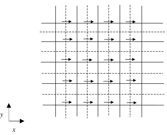
(1980). The problem is overcome by using a different set of points to calculate vectors and scalars. This is called the staggered grid concept where the calculation points for vectors are staggered with respect to the calculation points for scalars. Such a staggered grid for velocity components was first used by Harlow and Welch (1965).

In the staggered grid, the velocity components are calculated for the points that lie on the faces of a control volume. Thus, the x-component of velocity u is calculated at the faces that are normal to the x-direction. The locations for u are shown in Figure 2 by short arrows, while the grid points (hereafter called the main grid points) are shown by the intersections of the solid lines; the dashed lines indicate the control-volume faces.

x y

Figure 2. Staggered locations for u

Note that with respect to the main grid points, the u locations are staggered only in the x

Grids are developed, by using algebraic functions for grid spacing (non-uniform or uniform grid spacing). The staggered grid points are first developed. They are represented as xu(i) and yv(j)

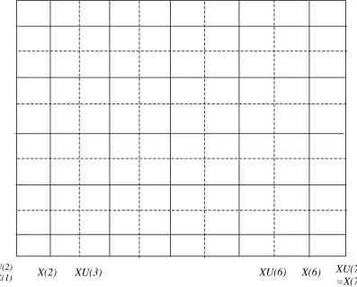
for x and y directions respectively. The main grid points are then calculated by using the staggered grid locations. Figure 3 shows the staggered and main grid locations xu(i) and x(i) respectively for the x direction on a 7x7 grid. Note that the boundary of the diagram is the physical boundary of the cavity. The staggered grid starts with xu(2) whereas the main grid starts with x(1). Note that xu(2)

= x(1) and xu(ni) = x(ni) with ni = 7. This representation allows the imposition of natural boundary

conditions for scalar and vector quantities. In the x direction, calculations for u velocity starts at

xu(3) and ends at xu(ni-1)=xu(6) whereas calculations for scalars and v velocity start at x(2) and

end at x(ni-1) = x(6). Similarly in the y direction, calculations for v velocity starts at yv(3) and ends

at yv(nj-1) = yv(6) whereas calculations for scalars and u velocity start at y(2) and end at y(nj-1) =

y(6).

XU(6) X(6) XU(7)

=X(7) XU(3)

X(2) XU(2)

=X(1)

The staggered grid generation is given as GRID GENERATION FUNCTIONS in SUBROUTINE READDATA and the development of the main grids from the staggered grids is shown as CALCULATE GEOMETRICAL QUANTITIES in SUBROUTINE INIT.

This part of the program is given below: NIM1=NI-1

NJM1=NJ-1 NIM2=NI-2 NJM2=NJ-2

C GRID GENERATION FUNCTIONS (development of the staggered grid. This is a part C of SUBROUTINE READDATA)

DO 101 I=2,NI

XU(I)=ELBYH*((I-2)/FLOAT(NIM2)-1/(2*3.14159)*SIN(2*3.14159*(I-2) 1/FLOAT(NIM2)))

101 CONTINUE DO 105 J=2,NJ

YV(J)=((J-2)/FLOAT(NJM2)-1/(2*3.14159)*SIN(2*3.14159*(J-2) 1/FLOAT(NJM2)))

105 CONTINUE

In the example presented above a sine function is used for generating the staggered grid in the x and y directions. This function can be expressed mathematically as:

( ) 2 1

sin 2

max 2 max

xu i i i

H i π π i

− ⎛

= − _⎜

⎝ ⎠

⎞

⎟ i=imin, imax

( ) 2 1

sin 2

max 2 max

yv j j i

H j π π i

− ⎛

= − _⎜

⎝ ⎠

⎞

⎟ j=jmin,jmax

where imin=jmin=2, imax=NI-2 and jmax=NJ-2 .

SUBROUTINE INIT INCLUDE 'common.h'

C CALCULATE GEOMETRICAL QUANTITIES X(1)=XU(2)

X(NI)=XU(NI) DO 101 I=2,NIM1

101 X(I)=0.5*(XU(I+1)+XU(I)) Y(1)=YV(2)

Y(NJ)=YV(NJ)

DO 102 J=2,NJM1

102 Y(J)=0.5*(YV(J+1)+YV(J)) DXPW(1)=0.0

C (DXPW(I), distance between two consecutive main grid points in the x-direction C starting from X(2) to X(NI))

DXEP(NI)=0.0

C (DXEP(I), distance between two consecutive main grid points in the x-direction C starting from X(1) to X(NIM1))

DO 103 I=1,NIM1 DXEP(I)=X(I+1)-X(I) 103 DXPW(I+1)=DXEP(I) DYPS(1)=0.0

C (DYPS(J), distance between two consecutive main grid points in the y-direction C starting from Y(2) to Y(NJ))

DYNP(NJ)=0.0

C (DYNP(J), distance between two consecutive main grid points in the y-direction C starting from Y(1) to Y(NJM1))

DXPWU(1)=0.0 DXPWU(2)=0.0

C (DXPWU(I), distance between two consecutive staggered grid locations in the x- C direction starting from XU(3) to XU(NI))

DXEPU(1)=0.0 DXEPU(NI)=0.0

C (DXEPU(I), distance between two consecutive staggered grid locations in the x- C direction starting from XU(2) to XU(NIM1))

DO 105 I=2,NIM1

DXEPU(I)=XU(I+1)-XU(I) 105 DXPWU(I+1)=DXEPU(I) DYPSV(1)=0.0

DYPSV(2)=0.0

C (DYPSV(J), distance between two consecutive staggered grid locations in the y- C direction starting from YV(3) to YV(NJ))

DYNPV(1)=0.0 DYNPV(NJ)=0.0

C (DYNPV(J), distance between two consecutive staggered grid locations in the y- C direction starting from YV(2) to YV(NJM1))

DO 106 J=2,NJM1 DYNPV(J)=YV(J+1)-YV(J)

106 DYPSV(J+1)=DYNPV(J) DO 107 I=1,NI

107 SEW(I)=DXEPU(I)

C (SEW(I), area associated with the non-staggered control volume in the x-direction) DO 108 J=1,NJ

108 SNS(J)=DYNPV(J)

C (SNS(J), area associated with the non-staggered control volume in the y-direction)

DO 109 I=1,NI 109 SEWU(I)=DXPW(I)

C (SEWU(I), area associated with the staggered control volume in the x-direction) DO 110 J=1,NJ

C (SNSV(J), area associated with the staggered control volume in the y-direction) As already mentioned the walls of the cavity are located at the staggered locations in order to facilitate the application of the no-slip and impermeable boundary conditions. Thus XU(2),

XU(NI), YV(2) and YV(NJ) are located on the cavity walls. The main grid locations, X(1), X(NI), Y(1) and Y(NJ) are set equal to XU(2), XU(NI), YV(2) and YV(NJ) respectively. X(1), X(NI), Y(1) and Y(NJ) are dummy points and are not used for calculations. Such an allocation also enables the use of natural boundary conditions for temperature at the wall. All other non-staggered locations are positioned in between the staggered locations.

Before carrying out calculations all the necessary data are read in by using SUBROUTINE READDATA. This subroutine in turn reads in the data file “IN.DAT”.

SUBROUTINE READDATA INCLUDE 'common.h'

C The include statement in FORTRAN does away with all common statements. This C information is stored in the include file common.h.

LOGICAL INCALU,INCALV,INCALP,INPRO,INCALK,INCALD,INCALM 1 ,INCALT,INHY,INCEN,STEADY

C These are logicals and are defined at the end of this listing. OPEN(2,FILE='in.dat')

C The file in.datcontains input parameters and is given in Section 17. C GRID, ITERATION AND COMPARISON PARAMETERS

READ(2,'(/////)')

READ(2,*)GREAT,NITER,SMALL,NFTSTP,NLTSTP,STEADY,TFIRST WRITE(*,*)"GREAT NITER SMALL NFTSTP NLTSTP STEADY TFIRST" WRITE(*,*)GREAT,NITER,SMALL,NFTSTP,NLTSTP,STEADY,TFIRST READ(2,*)

IF(STEADY)NFTSTP=1 IF(STEADY)NLTSTP=1 IF(STEADY) DT(1)=GREAT READ(2,*)IT,JT

READ(2,*)NSWPU,NSWPV,NSWPP,NSWPK,NSWPD,NSWPT WRITE(*,*)"NSWPU NSWPV NSWPP NSWPK NSWPD NSWPT" WRITE(*,*)NSWPU,NSWPV,NSWPP,NSWPK,NSWPD,NSWPT READ(2,'(/)')

READ(2,*)NI,NJ,ELBYH WRITE(*,*)"NI NJ ELBYH" WRITE(*,*)NI,NJ,ELBYH

C TIME STEP FOR UNSTEADY CALCULATIONS READ(2,'(/)')

READ(2,*)TSTEP WRITE(*,*)"TSTEP" WRITE(*,*)TSTEP

C DEPENDENT VARIABLE, DISCRETIZATION AND RESTART OPTIONS READ(2,'(/)')

READ(2,*)INCALU,INCALV,INCALP,INCALK,INCALD,INPRO,INCALT WRITE(*,*)"INCALU INCALV INCALP INCALK INCALD INPRO INCALT" WRITE(*,*)INCALU,INCALV,INCALP,INCALK,INCALD,INPRO,INCALT READ(2,*)

READ(2,*)INCALB,INHY,INCEN,VALUE WRITE(*,*)"INCALB INHY INCEN VALUE" WRITE(*,*)INCALB,INHY,INCEN,VALUE

C FLUID PROPERTIES

READ(2,'(/)')

READ(2,*)DENSIT,PRANDL,VISCOS,CPP WRITE(*,*)"DENSIT PRANDL VISCOS CPP" WRITE(*,*)DENSIT,PRANDL,VISCOS,CPP

C ALPHAF represents the thermal diffusivity of the fluid and is defined as

Pr

ρ µ α =

ALPHAF=VISCOS/(DENSIT*PRANDL)

C TURBULENCE CONSTANTS

READ(2,'(/)')

READ(2,*)CMU,CD,C1,C2,CAPPA,ELOG,PRTE,PRANDT

WRITE(*,*)"CMU CD C1 C2 CAPPA ELOG PRTE PRANDT" WRITE(*,*)CMU,CD,C1,C2,CAPPA,ELOG,PRTE,PRANDT READ(2,*)

READ(2,*)F1,F2 WRITE(*,*)"F1,F2" WRITE(*,*)F1,F2

PFUN=PRANDL/PRANDT

PFUN=9.24*(PFUN**0.75-1.0)*(1.0+0.28*EXP(-0.007*PFUN))

C BOUNDARY VALUES READ(2,'(/)')

READ(2,*)TH,TC WRITE(*,*)"TH TC" WRITE(*,*)TH,TC

C INTERNAL HEAT GENERATION AND RAYLEIGH NUMBER READ(2,'(/)')

READ(2,*)QGENER,RALI WRITE(*,*)"QGENER RALI" WRITE(*,*)QGENER,RALI

C TREF represents the reference temperature.

C BEITA represents β, the thermal expansion coefficient of the fluid. C DELT represents ∆T.

TREF=(TC+TH)/2

BEITA=1/(273.15+TREF) DELT=TH-TC

C PRESSURE CALCULATION

READ(2,'(/)')

READ(2,*)IPREF,JPREF WRITE(*,*)"IPREF JPREF" WRITE(*,*)IPREF,JPREF

C PROGRAM CONTROL AND MONITOR READ(2,'(/)')

READ(2,*)MAXIT,IMON,JMON,URFU,URFV WRITE(*,*)"MAXIT IMON JMON URFU URFV" WRITE(*,*)MAXIT,IMON,JMON,URFU,URFV READ(2,*)

READ(2,*)URFP,URFE,URFK,URFT WRITE(*,*)"URFP URFE URFK URFT" WRITE(*,*)URFP,URFE,URFK,URFT READ(2,*)

READ(2,*)URFG,URFVIS,INDPRI,SORMAX WRITE(*,*)"URFG URFVIS INDPRI SORMAX" WRITE(*,*)URFG,URFVIS,INDPRI,SORMAX

C CAVITY DIMENSIONS

EL=H*ELBYH

C GRID GENERATION FUNCTIONS NIM1=NI-1

NJM1=NJ-1 NIM2=NI-2 NJM2=NJ-2

DO 101 I=2,NI

XU(I)=ELBYH*((I-2)/FLOAT(NIM2)-1/(2*3.14159)*SIN(2*3.14159*(I-2) 1/FLOAT(NIM2)))

101 CONTINUE DO 105 J=2,NJ

YV(J)=((J-2)/FLOAT(NJM2)-1/(2*3.14159)*SIN(2*3.14159*(J-2) 1/FLOAT(NJM2)))

105 CONTINUE

C NON-DIMENSIONALISATION

C UREF represents uref, the reference value for velocity.

UREF=ALPHAF*(PRANDL*RALI)**0.5/H C R1 and R2 are the non-dimensional numbers given by

Ra Pr

and PrRa

R1=(PRANDL/RALI)**0.5 R2=(PRANDL*RALI)**0.5 CLOSE(2)

RETURN END

Following is a listing of the quantities read in from the input data file in.dat. C GREAT represents a large number that is sometimes used for comparison

or for some special purpose like assigning the boundary condition for ε=∞. C NITER represents the iteration counter for iterations in a single time step.

C SMALL represents a small number that is used for some special purpose in the program such as preventing division by zero.

C NLTSTP represents the last iteration step for time iterations.

C STEADY is a LOGICAL . IF STEADY is TRUE then the unsteady terms are omitted from the calculation procedure.

C TFIRST represents the starting value assigned to time t.

C IT and JT represent the maximum values that NI and NJ can have. If NI and NJ exceed the value of IT and JT respectively, new values have to be assigned to IT and JT. The program should then be recompiled.

C NSWPU, NSWPV, NSWPP, NSWPK, NSWPD, NSWPT are the total number of internal iterations used to calculate u, v, p’, k, εand T respectively.

C NI and NJ are the total number of grids in the x and y directions respectively. C ELBYH represents the ratio of length to height of the cavity.

C TSTEP represents the time step for unsteady calculations.

C LOGICALS INCALU, INCALV, INCALP, INCALK, INCALD, INPRO, INCALT activate SUBROUTINES CALCU, CALCV, CALCP, CALCTE, CALCED, PROPS, CALCT respectively.

C LOGICAL INCALB activates the buoyancy terms.

C LOGICALS INHY and INCEN activate the hybrid and central schemes respectively.

C If VALUE equals one, the program uses an initial field that has been fed in by the user. If VALUE equals zero, the program uses the solution that has been dumped in the DUMP file as the initial field. Thus for any fresh calculations, VALUE should always be one.

C DENSIT-fluid density. C PRANDL-fluid Prandtl number. C VISCOS-fluid viscosity.

C CMU-turbulence model constant, cµ. C CD-damping factor, fµ.

C C2-turbulence model constant, cε2.

C CAPPA-Von Karman’s constant, κ.

C ELOG- represents cκ where c is given by lnc=5.5 and κ is Von Karman’s constant. C PRTE-represents σκ.

C PRANDT-represents turbulent Prandtl number,σT.

C F1-damping factor, f1.

C F2-damping factor, f2.

C TH-temperature of the hot wall, Th.

C TC-temperature of the cold wall, Tc.

C QGENER-internal heat generation equals zero for the present problem. C CPP-specific heat of the fluid, CP.

C RALI-Rayleigh number.

C IPREF, JPREF-position of reference value for guessed pressure.

C MAXIT-maximum number of space iterations (i.e., number of iterations inside one time step).

C IMON, JMON- monitoring location for different variables. C URFU-under-relaxation factor for u.

C URFV-under-relaxation factor for v. C URFP-under-relaxation factor for p. C URFE-under-relaxation factor for ε. C URFK-under-relaxation factor for k. C URFT-under-relaxation factor for T.

C URFG-under-relaxation factor for µ/Pr or (µ+µt)/Pr.

C URFVIS-under-relaxation factor for µ or (µ+µt).

C INDPRI-number of iterations after which labels are printed on the screen. C SORMAX-convergence criterion.

The variables are initialized in SUBROUTINE INIT immediately after the subsection CALCULATE GEOMETRICAL QUANTITIES.

C UO(I,J), VO(I,J), PO(I,J), TO(I,J), TEO(I,J), EDO(I,J), DENO(I,J) represent the old value (i.e.,values at the previous time iteration for the respective variables)

DO 200 I=1,NI DO 200 J=1,NJ

C SMALL is used as an initial field to prevent division by zero. U(I,J)=SMALL

UO(I,J)=SMALL V(I,J)=SMALL VO(I,J)=SMALL P(I,J)=SMALL PO(I,J)=SMALL PP(I,J)=SMALL T(I,J)=0.5 TO(I,J)=0.5 TE(I,J)=SMALL TEO(I,J)=SMALL ED(I,J)=SMALL EDO(I,J)=SMALL DEN(I,J)=1.0+SMALL DENO(I,J)=1.0+SMALL VIS(I,J)=1.0+SMALL GAMH(I,J)=1.0+SMALL DU(I,J)=0.0

DV(I,J)=0.0

C DU(I,J) and DV(I,J) are quantities associated with the velocity correction equation. C The velocity correction equation is discussed in Section 9.

SU(I,J)=0.0

C SU(I,J) represents the overall source term and is equivalent to term b in Patankar C (1980).

SP(I,J)=0.0

C SP(I,J) represents SPin S=SC+SP.

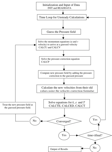
6. PROGRAM FLOW CHART

Time Loop for Unsteady Calculations

Guess the Pressure field

Solve the momentum equations (u and v

velocity) to arrive at a guessed velocity CALCU and CALCV

Solve the pressure correction equation CALCP

Compute new pressure field by adding the pressure correction to the guessed pressure

Calculate the new velocities from their old values using the velocity correction formulae

Solve equations for k, ε and T

CALCTE, CALCED, CALCT Treat the new pressure field as

the guessed pressure field.

No

Yes

Output of Results

Yes

No time<tfinal? Converged?

Figure 4. Flow chart explaining details of the solution procedure. (Names in block letters are those of subroutines.)

The SIMPLE algorithm which stands for Semi-Implicit Method for Pressure-Linked Equations is used for calculation of the flow field. The procedure has been described in Patankar and Spalding (1972). The flow chart described in Figure 4 gives a detailed description of the steps used in calculating the flow field along with the temperature field for the general unsteady turbulent solution. The pressure correction equation is used to incorporate the continuity equation in the solution procedure. The pressure correction equation is described in Section 9.

7. (SUBROUTINE LISOLV) THE GAUSS SEIDEL LINE BY LINE SOLVER

Including the pressure correction equation, there are now six partial differential equations to be solved. The following subroutines represent the six partial differential equations in their discretized form:

CALCU x-directional momentum equation

CALCV y-directional momentum equation

CALCP pressure correction equation

CALCTE equation for turbulence kinetic energy

CALCED equation for energy dissipation

CALCT thermal energy equation

These equations are solved by means of a line by line Gauss-Seidel solver that employs a combination of the Tri-Diagonal-Matrix Algorithm (TDMA) for one-dimensional situations and the point by point Gauss-Seidel iterative method.

Following is a description of the TDMA for one dimensional situations: The one dimensional discretized equation for a variable φcan be written as,

j j j j j j

j a b c

d φ = φ ₊₁+ φ ₋₁+ (14)

Where a, b, c and d represent coefficients of the discretized equation for variable φ. Subscript j

For the forward substitution process one seeks a relation,

j j j

j =Pφ +1+Q

φ (15)

With j=j-1 in the above relationship one can arrive at an equation for φ j-1,

1 1

1 − −

− = j j + j

j P φ Q

φ (16)

Substitution of Equation (16) into Equation (14) leads to,

(

j j j

)

j

j j j j

j a b P Q c

d φ = φ ₊₁+ ₋₁φ + ₋₁ + (17)

If Equation (17) is rearranged to take the form of Equation (15) and the coefficients are compared, one arrives at a recurrence relationship of the form,

1

−

− =

j j j

j j

P b d

a

P (18)

1 1

− −

− + =

j j j

j j j j

P b d

Q b c

Q (19)

For j=jmin, the recurrence relation (18) and (19) gives a definite value for Pminand Qmin.

Similarly for j=jmax, the recurrence relation gives a definite value for Pmax and Qmax. An

explanation for a specific boundary condition with temperature as the variable is given in Patankar (1980).

Summary of the algorithm

1. Calculate Pmin and Qmin using the left boundary conditions (i.e., for j=jmin)

2. Use the recurrence relations (18) and (19) to obtain Pj and Qjfor j=jmin+1, jmax.

3. Equate the right boundary conditions (i.e., for j=jmax) with Pmaxand Qmax.

4. Use Equation 15 for j=jmax-1, jmin to obtain φ jmax-1, φ jmin.

b a

a a

a

aPφP = EφE + WφW + NφN + SφS + (20)

where aP,aE, aW, aN and aS represent coefficients associated with the variable φ and b represents the

source term. In order to be able to use the TDMA one has to choose a particular direction for one sweep and assume the other direction to be a constant. In the present program, the S-N direction is chosen for calculations, and the W-E direction is assumed to be constant for every

sweep. Thus a new source term b0 is introduced as part of the terms in the W-E direction. Equation

(20) is thus modified into,

0

b a

a

a_Pφ_P = _Nφ_N + _Sφ_S + (21)

where b₀ =a_Eφ_E +a_Wφ_W +b.

Discussion on the line by line Gauss-Seidel method

The line by line scheme can be visualized with reference to Figure 5. The discretization equations for the grid points along a chosen line are considered first. These contain the values of φ at the grid points (shown by squares) along two adjacent lines. If these φ’s are substituted from their latest values, the equations for the grid points (shown by circles) along the chosen line would look like one-dimensional equations and could be solved by the TDMA. This procedure is carried out for all the lines in the S-N direction.

In the program, subroutine LISOLV represents the line by line Gauss-Seidel solver. SUBROUTINE LISOLV(ISTART,JSTART,NI,NJ,IT,JT,PHI)

DIMENSION PHI(IT,JT),A(90),B(90),C(90),D(90) COMMON

1/COEF/AP(80,80),AN(80,80),AS(80,80),AE(80,80),AW(80,80),SU(80,80), 1 SP(80,80)

NIM1=NI-1 NJM1=NJ-1

JSTM1=JSTART-1 A(JSTM1)=0.0

C COMMENCE W-E SWEEP DO 100 I=ISTART,NIM1 C(JSTM1)=PHI(I,JSTM1)

C COMMENCE S-N TRAVERSE DO 101 J=JSTART,NJM1

C ASSEMBLE TDMA COEFFICIENTS A(J)=AN(I,J)

C (A(J) represents aj in Equation (14))

B(J)=AS(I,J)

C (B(J) represents bjin Equation (14))

C(J)=AE(I,J)*PHI(I+1,J)+AW(I,J)*PHI(I-1,J)+SU(I,J) C (C(J) represents cj in Equation (14))

D(J)=AP(I,J)

C (D(J) represents dj in Equation (14))

C CALCULATE COEFFICIENTS OF RECURRENCE FORMULA TERM=1./(D(J)-B(J)*A(J-1))

A(J)=A(J)*TERM

101 C(J)=(C(J)+B(J)*C(J-1))*TERM

C The recurrence formulae (18) and (19) for Pjand Qj are stored in A(J) and C(J) here.

C OBTAIN NEW PHI"S DO 102 JJ=JSTART,NJM1 J=NJ+JSTM1-JJ

100 CONTINUE RETURN END

8. SUBROUTINE CALCU AND CALCV (MOMENTUM EQUATIONS)

Subroutines CALCU and CALCV representing the discretized form of the momentum equations are described here. The momentum equation in the x direction can be written as:

(

)

(

)

⎥ ⎦ ⎤ ⎢ ⎣ ⎡ ⎟⎟ ⎠ ⎞ ⎜⎜ ⎝ ⎛ ∂ ∂ + ∂ ∂ + ∂ ∂ + ⎥ ⎦ ⎤ ⎢ ⎣ ⎡ ⎟ ⎠ ⎞ ⎜ ⎝ ⎛ ∂ ∂ + ∂ ∂ + ∂ ∂ − = ∂ ∂ + ∂ ∂ + ∂ ∂ x v y u y Ra Pr x u 2 x Ra Pr x p y u v x u u t u t

t µ µ

µ µ ρ

ρ ρ

Modifying the diffusion term on the right hand side one can rewrite the equation as follows:

(

)

(

)

_⎥+ ⎦ ⎤ ⎢ ⎣ ⎡ ∂ ∂ + ∂ ∂ + ⎥⎦ ⎤ ⎢⎣ ⎡ ∂ ∂ + ∂ ∂ + ∂ ∂ − = ∂ ∂ + ∂ ∂ + ∂ ∂ y u y Ra Pr x u x Ra Pr x p y u v x u u t u t

t µ µ

µ µ ρ ρ ρ

(

)

⎥ ⎦ ⎤ ⎢ ⎣ ⎡ ⎟⎟ ⎠ ⎞ ⎜⎜ ⎝ ⎛ ∂ ∂ + ∂ ∂ + ∂ ∂ y v x u x Ra Pr t µ

µ (22)

For an incompressible fluid since the density does not change with time, the term:

(

)

_⎥ ⎦ ⎤ ⎢ ⎣ ⎡ ⎟⎟ ⎠ ⎞ ⎜⎜ ⎝ ⎛ ∂ ∂ + ∂ ∂ + ∂ ∂ y v x u x Ra Pr t µ

µ (22a)

equals zero due to continuity. The retention of this term increases the numerical accuracy in some types of flows. Therefore this term is included in our formulation as a source term. For a

description of the discretization procedure one can refer to Patankar (1980). The initial and final discretized forms in two dimensions is presented here.

Initial discretized form:

y x ) u S S ( J J J J t y x ) u u ( P P C s n w e o P o P P

P ∆ ∆

∆ ∆ ∆ ρ ρ + = − + − + − (23) where ( ) ( )

e e t e

u

J u u

x

ρ µ µ ∂

⎧ ⎫

=_⎨ − + _⎬

∂

( ) ( )

w w t w

u

J u u

x

ρ µ µ ∂

⎧ ⎫

=_⎨ − + _⎬

∂

⎩ ⎭∆y

( ) ( )

n n t n

u

J v u

y

ρ µ µ

⎧ ∂ ⎫

=_⎨ − + _⎬

∂

⎩ ⎭∆x

( ) ( )

s s t s

u

J v u

y

ρ µ µ

⎧ ∂ ⎫

=_⎨ − + _⎬

∂

⎩ ⎭∆x

P p

C S u

S

S = + represents the source term. Terms arising due to the non-dimensional form have been omitted for ease of understanding. The old values (i.e., the values at the beginning of the time step) are denoted by the superscript o.

Final discretized form:

b u a u a u a u a u

a_{P P} = _{E E} + _{W W} + _{N N} + _{S S} + (24)

where

( )

P

[[

F ,0 A

D

a_E = _{e e} + − _e

]]

( )

P

[[

F ,0 A

D

a_W = _{w w} + _w

]]

( )

P

[[

F ,0 A

D

a_N = _{n n} + − _n

]]

( )

P

[[

F ,0 A

D

a_S = _{s s} + _s

]]

{The symbol

[ ]

[ ]

represents the largest of the quantity contained within it}

t y x a o P o P _∆ ∆ ∆ ρ = M u a y x S

b= _C∆ ∆ + _Po _Po +

(24a) y x S a a a a a

a_P = _E + _W + _N + _S + o_P − _P∆ ∆

with F_e =(ρu)_e∆y,

e e t e ) x ( y ) ( D δ ∆ µ µ+ = , e e e D F P = y ) u (

F_w = ρ _w∆ ,

w w t w ) x ( y ) ( D δ ∆ µ µ+ = , w w w D F P = x ) v (

F_n = ρ _n∆ ,

n n t n ) y ( x ) ( D δ ∆ µ µ + = , n n n D F P = x ) v (

F_s = ρ _s∆ ,

s s t s ) y ( x ) ( D δ ∆ µ µ + = , s s s D F P =

( )

P

A represents a function which assumes different forms for different discretization schemes. The central difference scheme and the hybrid scheme are used in the present program.

N

S W

Control volume

∆x

∆y

Js Jn

Jw Je

w e

n

s

y

x

P E

Figure 6. Control volume for a two-dimensional situation.

Other schemes include the upwind scheme, the power law scheme, the exponential or exact scheme and are described in detail in Patankar (1980) and the QUICK scheme of Leonard (1979). The term M in the source term represents modifications to the momentum equation such as the inclusion of the term (22a). The eddy viscosity µtis represented with the help of a modification to

SUBROUTINE CALCU INCLUDE 'common.h'

LOGICAL INHY,INCEN,STEADY

C Note that I starts from 3. Due to staggering, I=2 represents dummy points. DO 100 I=3,NIM1

DO 101 J=2,NJM1

C COMPUTE AREAS AND VOLUME AREANS=SEWU(I)

C represents staggered area in the x-direction and applies to fluid in the y-direction AREAEW=SNS(J)

C represents non-staggered area in the y-direction and applies to fluid in the x-direction VOL=SEWU(I)*SNS(J)

C represents the control volume.

C CALCULATE CONVECTION COEFFICIENTS

C represents F in Equations (24a). Note that the variables are to be evaluated at the C faces of the control volume. The U velocity is staggered in the x-direction. Thus C the appropriate interpolated values for V velocity and density need to be taken. GN=0.5*(DEN(I,J+1)+DEN(I,J))*V(I,J+1)

GNW=0.5*(DEN(I-1,J)+DEN(I-1,J+1))*V(I-1,J+1) GS=0.5*(DEN(I,J-1)+DEN(I,J))*V(I,J)

GSW=0.5*(DEN(I-1,J)+DEN(I-1,J-1))*V(I-1,J) GE=0.5*(DEN(I+1,J)+DEN(I,J))*U(I+1,J) GP=0.5*(DEN(I,J)+DEN(I-1,J))*U(I,J) GW=0.5*(DEN(I-1,J)+DEN(I-2,J))*U(I-1,J)

CN=0.5*(GN+GNW)*AREANS CS=0.5*(GS+GSW)*AREANS CE=0.5*(GE+GP)*AREAEW CW=0.5*(GP+GW)*AREAEW

C CALCULATE DIFFUSION COEFFICIENTS

C represents D in Equations (24a). Appropriate interpolated values need to be taken C for viscosity, VIS(I,J). VIS(I,J) represents either the fluid viscosity (laminar C flow) or the total of fluid viscosity and eddy viscosity (turbulent flow). R1 C represents the factor

Ra Pr

VISS=0.25*(VIS(I,J)+VIS(I,J-1)+VIS(I-1,J)+VIS(I-1,J-1)) DN=R1*VISN*AREANS/DYNP(J)

DS=R1*VISS*AREANS/DYPS(J) DE=R1*VIS(I,J)*AREAEW/DXEPU(I) DW=R1*VIS(I-1,J)*AREAEW/DXPWU(I)

C CALCULATE COEFFICIENTS OF SOURCE TERMS

C the coefficients of the source term S=SC+SPuP are calculated here

C CPO*U(I,J) represents S_C∆x∆y and SP(I,J) represents S_P∆x∆y

SMP=CN-CS+CE-CW CP=AMAX1(0.0,SMP) CPO=CP

C ASSEMBLE MAIN COEFFICIENTS

C the main coefficients aE, aW, aN and aS are evaluated depending on the type of

C discretization used. The hybrid scheme (INHY) or the central scheme C (INCEN) is used here.

C For the hybrid scheme the function A

( )

P =

[

[

0,1−0.5P

]

]

IF (INHY) THEN

AN(I,J)=DN*AMAX1(0.,1-0.5*ABS(CN/DN))+AMAX1(-CN,0.) AS(I,J)=DS*AMAX1(0.,1-0.5*ABS(CS/DS))+AMAX1(CS,0.) AE(I,J)=DE*AMAX1(0.,1-0.5*ABS(CE/DE))+AMAX1(-CE,0.) AW(I,J)=DW*AMAX1(0.,1-0.5*ABS(CW/DW))+AMAX1(CW,0.) END IF

C For the central scheme the function A

( )

P =1−0.5P

IF (INCEN) THEN

AN(I,J)=AMAX1(-CN,0.)+DN-0.5*ABS(CN) AS(I,J)=AMAX1(CS,0.)+DS-0.5*ABS(CS) AE(I,J)=AMAX1(-CE,0.)+DE-0.5*ABS(CE) AW(I,J)=AMAX1(CW,0.)+DW-0.5*ABS(CW) END IF

C Logical STEADY =TRUE implies that the steady state problem is solved and C the unsteady term

t u

∂ ∂

ρ is omitted.

APO(I,J)=0.0 ELSE

APO(I,J)=DEN(I,J)*VOL/DT(ITSTEP) END IF

C The pressure gradient is not included in the momentum source term S=SC+SPuP.

C This is because the pressure field needs to be ultimately calculated . C Thus the pressure gradient is included as a separate source term in SU(I,J). C It is given here as DU(I,J)*(P(I-1,J)-P(I,J)).

C (Refer to Section 9 for the pressure correction equation.) DU(I,J)=AREAEW

SU(I,J)=CPO*U(I,J)+DU(I,J)*(P(I-1,J)-P(I,J))+APO(I,J)*UO(I,J) SP(I,J)=-CP

C Extra term to improve numerical stability:

(

)

⎥

⎦ ⎤ ⎢

⎣ ⎡

⎟⎟ ⎠ ⎞ ⎜⎜

⎝ ⎛

∂ ∂ + ∂ ∂ + ∂

∂

y v x u x

Ra Pr

t

µ µ

DUDXP =(U(I+1,J)-U(I,J))/DXEPU(I) DUDXM =(U(I,J)-U(I-1,J))/DXPWU(I)

SU(I,J)=R1*(VIS(I,J)*DUDXP-VIS(I-1,J)*DUDXM)/SEWU(I)*VOL+SU(I,J) GAMP =0.25*(VIS(I,J)+VIS(I-1,J)+VIS(I,J+1)+VIS(I-1,J+1))

DVDXP =(V(I,J+1)-V(I-1,J+1))/DXPW(I)

GAMM =0.25*(VIS(I,J)+VIS(I-1,J)+VIS(I,J-1)+VIS(I-1,J-1)) DVDXM =(V(I,J)-V(I-1,J))/DXPW(I)

SU(I,J) =SU(I,J)+R1*(GAMP*DVDXP-GAMM*DVDXM)/SNS(J)*VOL 101 CONTINUE

100 CONTINUE

C ENTRY MODU in SUBROUTINE PROMOD contains information about the C boundary conditions for u-velocity (Section 14).

CALL MODU

C The residual source term RESORU gives an idea about the convergence of the C solution. RESORU is the difference in the total source term between two C consecutive iteration steps.

RESORU=0.0 DO 300 I=3,NIM1 DO 301 J=2,NJM1

RESOR=AN(I,J)*U(I,J+1)+AS(I,J)*U(I,J-1)+AE(I,J)*U(I+1,J) 1 +AW(I,J)*U(I-1,J)-AP(I,J)*U(I,J)+SU(I,J)

VOL=SEW(I)*SNS(J) SORVOL=GREAT*VOL

IF(-SP(I,J).GT.0.5*SORVOL) RESOR=RESOR/SORVOL RESORU=RESORU+ABS(RESOR)

C UNDER-RELAXATION

C In an iterative procedure it is often desirable to speed up or slow down changes in C the dependent variable from iteration to iteration in order to avoid divergence. C The former is achieved by over-relaxation and the latter is achieved by under- C relaxation. The under-relaxation method is used in the present program. URFU C represents the under-relaxation factor used for the u-velocity. The value of under- C relaxation factor is always between 0 and 1.

AP(I,J)=AP(I,J)/URFU

SU(I,J)=SU(I,J)+(1.-URFU)*AP(I,J)*U(I,J) DU(I,J)=DU(I,J)*URFU

301 CONTINUE 300 CONTINUE

C SUBROUTINE LISOLV (Section 7) is used to solve the x-directional momentum C equation. NSWPU represents the number of internal iterations used for u.

DO 400 N=1,NSWPU

400 CALL LISOLV(3,2,NI,NJ,IT,JT,U) RETURN

END

The subroutine used to calculate the y-directional momentum equation, CALCV, is very similar to CALCU. However one has to remember that the calculation points for v velocity are staggered in the y-direction. An extra source term is added to b in the form of the buoyancy term. Following is a listing of SUBROUTINE CALCV.

SUBROUTINE CALCV INCLUDE 'common.h'

LOGICAL INCALB,INHY,INCEN,STEADY

DO 101 J=3,NJM1

C COMPUTE AREAS AND VOLUME AREANS=SEW(I)

C represents non-staggered area in the x-direction and applies to fluid in the y-direction. AREAEW=SNSV(J)

C represents staggered area in the y-direction and applies to fluid in the x-direction. VOL=SEW(I)*SNSV(J)

C CALCULATE CONVECTION COEFFICIENTS GN=0.5*(DEN(I,J+1)+DEN(I,J))*V(I,J+1)

GP=0.5*(DEN(I,J)+DEN(I,J-1))*V(I,J) GS=0.5*(DEN(I,J-1)+DEN(I,J-2))*V(I,J-1) GE=0.5*(DEN(I+1,J)+DEN(I,J))*U(I+1,J)

GSE=0.5*(DEN(I,J-1)+DEN(I+1,J-1))*U(I+1,J-1) GW=0.5*(DEN(I,J)+DEN(I-1,J))*U(I,J)

GSW=0.5*(DEN(I,J-1)+DEN(I-1,J-1))*U(I,J-1) CN=0.5*(GN+GP)*AREANS

CS=0.5*(GP+GS)*AREANS CE=0.5*(GE+GSE)*AREAEW CW=0.5*(GW+GSW)*AREAEW

C CALCULATE DIFFUSION COEFFICIENTS

VISE=0.25*(VIS(I,J)+VIS(I+1,J)+VIS(I,J-1)+VIS(I+1,J-1)) VISW=0.25*(VIS(I,J)+VIS(I-1,J)+VIS(I,J-1)+VIS(I-1,J-1)) DN=R1*VIS(I,J)*AREANS/DYNPV(J)

DS=R1*VIS(I,J-1)*AREANS/DYPSV(J) DE=R1*VISE*AREAEW/DXEP(I) DW=R1*VISW*AREAEW/DXPW(I)

C CALCULATE COEFFICIENTS OF SOURCE TERMS SMP=CN-CS+CE-CW

CP=AMAX1(0.0,SMP) CPO=CP

C ASSEMBLE MAIN COEFFICIENTS IF (INHY) THEN

AN(I,J)=DN*AMAX1(0.,1-0.5*ABS(CN/DN))+AMAX1(-CN,0.) AS(I,J)=DS*AMAX1(0.,1-0.5*ABS(CS/DS))+AMAX1(CS,0.) AE(I,J)=DE*AMAX1(0.,1-0.5*ABS(CE/DE))+AMAX1(-CE,0.) AW(I,J)=DW*AMAX1(0.,1-0.5*ABS(CW/DW))+AMAX1(CW,0.) END IF

IF (INCEN) THEN

AW(I,J)=AMAX1(CW,0.)+DW-0.5*ABS(CW) END IF

IF(STEADY) THEN APO(I,J)=0.0

ELSE

APO(I,J)=DEN(I,J)*VOL/DT(ITSTEP) END IF

DV(I,J)=AREANS

SU(I,J)=CPO*V(I,J)+DV(I,J)*(P(I,J-1)-P(I,J))+APO(I,J)*VO(I,J)

C BUOYANCY TERM

C Buoyancy term is included as a source term in SU(I,J). The reference C temperature, TREF, is given the value 0.5 which represents (Th+Tc)/2.

C Depending on the value assigned to TREF the approach to a steady solution would be C different. However the final steady solution will always remain the same. Note that the C temperature, T, has an interpolated value in the buoyancy term BOUYA to account for the C staggering.

TREF=0.0

IF (INCALB) THEN

BOUYA=(0.5*(T(I,J)+T(I,J-1))-TREF) SU(I,J)=SU(I,J)+BOUYA*VOL END IF

SP(I,J)=-CP

C Extra term to improve numerical stability:

(

)

_⎥

⎦ ⎤ ⎢

⎣ ⎡

⎟⎟ ⎠ ⎞ ⎜⎜

⎝ ⎛

∂ ∂ + ∂ ∂ + ∂

∂

y v x u x

Ra Pr

t

µ µ

DUDYP =(U(I+1,J)-U(I+1,J-1))/DYPS(J)

GAMP =0.25*(VIS(I,J)+VIS(I+1,J)+VIS(I,J-1)+VIS(I+1,J-1)) GAMM =0.25*(VIS(I,J)+VIS(I-1,J)+VIS(I,J-1)+VIS(I-1,J-1)) DUDYM =(U(I,J)-U(I,J-1))/DYPS(J)

SU(I,J)=SU(I,J)+R1*(GAMP*DUDYP-GAMM*DUDYM)/SEW(I)*VOL DVDYP =(V(I,J+1)-V(I,J))/DYNPV(J)

RGAMP =VIS(I,J)

DVDYM =(V(I,J)-V(I,J-1))/DYPSV(J) RGAMM =VIS(I,J-1)

SU(I,J) =SU(I,J)+R1*(RGAMP*DVDYP-RGAMM*DVDYM)/SNSV(J)*VOL 101 CONTINUE

100 CONTINUE

CALL MODV

C RESORV represents the residual source term for the y-directional momentum C equation.

RESORV=0.0 DO 300 I=2,NIM1 DO 301 J=3,NJM1

AP(I,J)=AN(I,J)+AS(I,J)+AE(I,J)+AW(I,J)+APO(I,J)-SP(I,J) DV(I,J)=DV(I,J)/AP(I,J)

RESOR=AN(I,J)*V(I,J+1)+AS(I,J)*V(I,J-1)+AE(I,J)*V(I+1,J) 1 +AW(I,J)*V(I-1,J)-AP(I,J)*V(I,J)+SU(I,J)

VOL=SEW(I)*SNS(J) SORVOL=GREAT*VOL

IF(-SP(I,J).GT.0.5*SORVOL) RESOR=RESOR/SORVOL RESORV=RESORV+ABS(RESOR)

C UNDER-RELAXATION

C URFV represents under-relaxation factor for v velocity. AP(I,J)=AP(I,J)/URFV

SU(I,J)=SU(I,J)+(1.-URFV)*AP(I,J)*V(I,J) DV(I,J)=DV(I,J)*URFV

301 CONTINUE 300 CONTINUE

C Subroutine LISOLV (Section7) is used to solve the y-directional momentum equation. C NSWPV represents the number of internal iterations used for v.

DO 400 N=1,NSWPV

400 CALL LISOLV(2,3,NI,NJ,IT,JT,V) RETURN

END

9. SUBROUTINE CALCP (THE PRESSURE CORRECTION EQUATION)

The continuity equation is included in the solution procedure through the introduction of the pressure correction equation in case of the SIMPLE ALGORITHM that is used in the present program. A relationship between pressure and velocity is derived. This is used in the continuity equation to derive the pressure correction equation. A detailed derivation of the pressure correction equation is given in Patankar (1980). The main steps in the derivation are given here.

(25)

' *

p p p= +

A similar equation can be written for the corrected velocities, u and v:

, (26)

'

* _u

u

u= + v=v* +v'

where u* and v* are the guess velocities and u’ and v’ are the velocity corrections. The velocity correction formulae can be written as:

, (27)

) p p ( d

u' = _{w W}' − '_P v' =d_s(p'_S − p'_P )

where

P ew w

a A

d = and

P ns s

a A

d = .

Aewand Ans represent areas associated with the East-West and North-South directions respectively.

In Patankar (1980) a slightly different formulation is given for the velocity correction formulae but both the formulations have the same meaning. Thus Equation (27) gives a relationship between the velocity correction and pressure correction. One can now write Equation (26) as follows:

, (28)

) p p ( d u

u= * + _{w W}' − '_P v=v* +d_s(p'_S − p'_P )

The continuity equation can be written as:

0 y

) v ( x

) u (

t ∂ =

∂ + ∂ ∂ + ∂

∂ρ ρ ρ

(29)

This equation is integrated over the shaded control volume in Figure 7.

For the integration of the term

t

∂

∂ρ _{, the density,}

P

ρ , is assumed to prevail over the control volume. Since a fully implicit procedure is used for time, the new values of velocity and density (i.e., those at time t+∆t) are assumed to prevail over the time step; the old density, (i.e., at time t), will appear only through the term

o P

ρ

t

∂ ∂ρ