TIME SERIES ANALYSIS ON EXPORTS AND ITS DETERMINANTS
Dr.P.Ambiga Devi, Professor of Economics
Dr.S.Gandhimathi, Associate Professor of Economics,
Institute for Home Science and Higher Education for Women, Coimbatore 641 043
1991-2012.The study was carried out in four sections. Section I briefly introduces the topic taken for the work. Section II gives a brief analysis on the various studies so far have been undertaken in India on the determinants of exports. Section III states the methodology adopted for the study. Section IV discusses the findings of the study and section V gives the conclusions emerging from the findings of the study.
Section II
Earlier studies on exports
Using the Granger (1969), Sims (1972) and Hsiao (1987) causality procedures export led growth hypothesis was tested in a number of studies (Jung and Marshall, 1985; Chow, 1987; Darrat, 1987; Hsiao, 1987; Bahmani- Oskooee et al, 1991; Kugler, 1991; Dodaro, 1993; Vanden Berg Schmidi, 1994; Greenway and Sapasford(1994) and Islam, 1998). But these studies failed to provide an unvarying conclusion between export growth and output growth.
Number of studies has been carried out for testing the causality between exports and economic growth for Indian data also. Mishra reinvestigated the dynamics of the relationship between exports and economic growth for India over the period 1970 to 2009. Applying popular time series econometric techniques of cointegration and vector error correction estimation, the study provides the evidence of stationarity of time series variables, existence of long-run equilibrium relation between them, and finally, the rejection of export-led growth hypothesis for India by the Granger causality test based on vector error correction model estimation.
Barua (2013) studied the cointegration between FDI, GDP and exports for India for the period 2000-2012. The findings of the study clearly indicated the significant relationship between the three variables. It revealed that 1 % increase in FDI could cause 4.7 %increase in exports.
Pathania Rajni( 2013) studied the linkages between export, import and capital formation applying time series econometric techniques like unit root test, co-integration and Granger causality for the period 1991 to 2010 for India. This study checked whether there is uni-directional or bidirectional causality between export, import and capital formation in India. In this paper, the results revealed that there is bidirectional causality between gross domestic capital formation and export growth. The traditional Granger causality test also suggested the uni-directional causality between capital formation and import and export.
causality approach. Annual time series data on India for the variables exports and GDP per capita stemming from 1980 to 2012 were used in the analysis. The tests on the long run and short run relationship between exports and economic growth are conducted. Based on the findings of cointegration approach this paper concluded that there does not exist long run equilibrium relationship between exports and GDP per capita. Granger causality test exhibits bidirectional causality running from exports to GDP per capita and GDP per capita to exports.
Anwar and Sampath (2000) examined the export-led growth hypothesis for 97 countries (including India, Pakistan and Sri Lanka) for the period 1960 to 1992. They found the evidence of unidirectional causality in the case of Pakistan and Sri Lanka, and no causality in the case of India. However, Kemal et al (2002) found a positive association between exports and economic growth for India as well as for other economies of South Asia. In the case of India, Chandra (2000; 2002) found bi-directional causal relationship between growth of exports and GDP growth which is a short-run causal relation, as cointegration between growth of exports and GDP growth was not found. Sharma and Panagiotidis (2004) tested the export-led growth hypothesis in the context of India, and the results strengthen the arguments against the export-led growth hypothesis for the case of India. Raju and Kurien (2005) analyzed the relationship between exports and economic growth in India over the pre-liberalization period 1960-1992, and found strong support for unidirectional causality from exports to economic growth using Granger causality regressions based on stationary variables, with and without an error-correction term. Dash (2009) analyzed the causal relationship between growth of exports and economic growth in India for the post-liberalization period 1992-2007, and the results indicate that there exists a long-run relationship between output and exports, and it is unidirectional, running from growth of exports to output growth.
Section III
Data and Methodology
methodology employed in this study is the cointegration and error correction modeling technique. The entire estimation procedure consists of three steps: first, unit root test; second, cointegration test; and the third, the error correction model estimation.
3.1 Unit Root Test
The econometric methodology first examines the stationarity properties of each time series of consideration. The present study uses Augmented Dickey-Fuller (ADF) unit root test to examine the stationarity of the data series. It consists of running a regression of the first difference of the series against the series lagged once, lagged difference terms and optionally, a constant and a time trend. This can be expressed as follows:
ΔYt = α0 + α1 t + α 2 Yt-1+ ∑ αjΔYt-j +€t
The additional lagged terms are included to ensure that the errors are uncorrelated. In this ADF procedure, the test for a unit root is conducted on the coefficient of Yt-1 in the regression. If the coefficient is significantly different from zero, then the hypothesis that Yt contains a unit root is rejected. Rejection of the null hypothesis implies stationarity. Precisely, the null hypothesis is that the variable Yt is a non-stationary series (H0: α2 =0) and is rejected when α2 is significantly negative (Ha: α2‹ 0). If the calculated value of ADF statistic is higher than McKinnon’s critical values, then the null hypothesis (H0) is not rejected and the series is non-stationary or not integrated of order zero, I(0). Alternatively, rejection of the null hypothesis implies stationarity. Failure to reject the null hypothesis leads to conducting the test on the difference of the series, so further differencing is conducted until stationarity is reached and the null hypothesis is rejected. If the time series (variables) are non-stationary in their levels, they can be integrated with I(1), when their first differences are stationary.
3.2 Cointegration Test
likelihood procedure. In the Johansen framework, the first step is the estimation of an unrestricted, closed p order VAR in
K variables.
3.3 Vector Error Correction Model (VECM)
Once the cointegration is confirmed to exist between variables, then the third step entails the construction of error correction mechanism to model dynamic relationship. The purpose of the error correction model is to indicate the speed of adjustment from the short-run equilibrium to the long-run equilibrium state. A Vector Error Correction Model (VECM) is a restricted VAR designed for use with non-stationary series that are known to be cointegrated. Once the equilibrium conditions are imposed, the VECM describes how the examined model is adjusting in each time period towards its long-run equilibrium state. Since the variables are supposed to be cointegrated, then in the short-run, deviations from this long-run equilibrium will feedback on the changes in the dependent variables in order to force their movements towards the long-run equilibrium state. Hence, the cointegrated vectors from which the error correction terms are derived are each indicating an independent direction where a stable meaningful long-run equilibrium state exists. The VECM has cointegration relations built into the specification so that it restricts the long-run behavior of the endogenous variables to converge on their cointegrating relationship while allowing for short-run adjustment dynamics.
Section IV
Results and Discussion
As the study was based on time series data for the period 1991-2012, it was necessary to test the stationarity of the variables in the export equation. Dickey Fuller statistics (Unit root test) was first applied to test for the stationarity of the chosen variables. After checking for stationarity, the long run relationship between exports and the selected variables. Viz, foreign direct investment, exchange rate and investment on infrastructure was established by estimating the error correction model.
All the variables in the model were tested for stationarity using unit root test with and without trend. The null hypothesis tested was
HO: Xit is non stationary Ha: Xit is stationary.
Without trend
Ln Xit = ao + a1 Ln Xit-1 +Uit
With trend
Ln Xit = ao + a1 Ln Xit-1 +Ln t +Uit
The ‘tau’ statistics for the coefficients were calculated. If the calculated ‘tau’ value is greater than the DF critical value the time series is stationary, otherwise not. The computed ‘tau’ statistics are shown in Table 1
TABLE-1
‘tau’ STATISTICS- DICKEY FULLER TEST
Figures in parentheses indicate t values
The table reveals that the variables exports, exchange rate and investment in infrastructure were statistically insignificant at 5% level when tested with trend. It indicated the acceptance of the null hypothesis of presence of unit root in the above stated variables which implies that these variables were non stationary at zero level of difference. The variable foreign direct investment was statistically significant and was stationary at zero level of difference. The stationarity of all the variables in same order of difference is essential for estimating a non spurious regression equation. Hence, they were put into different levels of stationary process to find out the order of difference in which all the variables were stationary. The following Table -2 shows the order of difference in which the variables were stationary.
Variables without
trend
Significance at 5% level
with trend
Significance at 5% level
Exports 0.0177
(0.5475)
In significant -0.2349 (-1.6233)
In significant Foreign Direct Investment -0.1717
(-3.3036)
Significant -0.4391 (-3.1402)
Significant
Exchange rate -0.1911
(-3.0920)
Insignificant 0.2982 (2.9847)
In significant Investment in
infrastructure
0.0567 (1.2125)
In significant -0.0877 (-0.7418)
TABLE-2
ORDER OF DIFFERENCE AND ‘tau’ STATISTICS– AUGUMENTED DICKY FULLER TEST
Figures in parentheses denote t values
The Augmented Dickey Fuller ‘tau’ statistics were calculated at first order difference and were found to be statistically significant. Hence all the selected variables were stationary at first order difference.
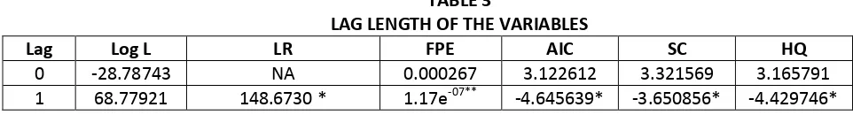
To calculate the long run relationship between the variables, the determination of lag length is essential. The sequential LR Statistic, Final Prediction Error test, Akaike Information Criterion, Schwarz Information Criterion and Hannan – Quinn Information Criterion were used to identify the lag length of the variables and the calculated lag length for the variables are given in Table 3
TABLE 3
LAG LENGTH OF THE VARIABLES
Lag Log L LR FPE AIC SC HQ
0 -28.78743 NA 0.000267 3.122612 3.321569 3.165791
1 68.77921 148.6730 * 1.17e-07** -4.645639* -3.650856* -4.429746* All the above said variables in the identification of lag length were statistically insignificant at zero lag. But at lag length one, using Sequential LR Statistic, Final Prediction Error Test, Akaike Information Criteria, Schwarz Information Criterion and Hannan – Quinn Information Criterion they were found to be statistically significant. It implied that at lag length one all the variables were to be selected for the vector error correction model.
Variables Order of
difference without trend
Significance at 5% level
with trend Significance at
5% level
Export First order 1.076038
(-4.3909)
Significant 1.167018 (-4.4643)
Significant Foreign Direct
Investment
First order -0.806778 (-3.735230)
Significant -0.915642 (-3.9801)
Significant
Exchange rate First order -0.869820 (-3.7132)
Significant -1.018063 (-3.6584)
Significant
Infrastructure First order -0.869820 (-3.7132)
Significant -1.018063 ( 3.7066)
In case of non stationary data it is quite possible that there is a linear combination of integrated variables that is stationary. Such variables are said to be co integrated. To understand the Co integrating relationship across these variables, the study uses Johansen (1991) Co integration Test. Using the Johansen (1991) co integration test, the unrestricted co integration trace test and maximum eigen value test were calculated.
TABLE - 4
UNRESTRICTED COINTEGRATION - MAX-EIGEN VALUE TEST
In both unrestricted co integration trace test and unrestricted co integration - max Eigen value test, the null hypothesis of no co integration was rejected at the 0.05 level (75.01204 > 47.85613 and 44.0409 > 27.58434). But the null hypothesis of one co integration among the variables is not rejected at the 0.05 level (27.9786< 29.79707 and 0.527668 < 21.13162) by both the trace statistics and max- Eigen statistics respectively. Hence, the Johansen methodology concludes there exist one co integrating relationship among the selected variables. So, estimation of Vector Error Correction Model is required in this context.
ESTIMATION OF LONG RUN RELATIONSHIP – VECTOR ERROR CORRECTION MODEL
The current investment on infrastructure and exchange did not exhibit short relation with exports, exchange rate. The long run relationship between exports and foreign direct investment, infrastructure, exchange rate for the period 1991 -2012 are shown in the Table.
Hypothesized
No. of CE(s) Eigen value
Max-Eigen Statistic
0.05
Critical Value Prob.**
None * None * 44.0409 43.65192 27.58434
At most 1 * At most 1 0.527668 15.00146 21.13162
At most 2 * At most 2 0.466057 12.54932 14.26460
At most 3 At most 3 0.173426 3.809326 3.841466
Max-eigen value test indicates 1 co integrating eqn (s) at the 0.05 level * denotes rejection of the hypothesis at the 0.05 level
TABLE -5
IMPACT OF
FOREIGN DIRECT
INVESTMENT ON EXPORT –ERROR CORRECTION MODEL
*statistically significant. Figures in( ) denotes standard error and figures in [ ]denote t values
The vector error correction model shows that the one year lagged investment on infrastructure development and the exchange rate were statistically significant at five percent level. The significance of lagged variables indicates long run relationship between exports and investment on infrastructure development and exchange rate. The lagged investment on infrastructure and exchange rate had increased the export of India. The lagged impact of FDI on exports was statistically in significant. But the current foreign direct investment was statistically significant. It means the there was no long relationship between foreign direct investment and value of export.
C -5.028153
Export(-1) 1.00000
Exchange rate(-1)
1.102524* (0.29288) [ 3.76442]
Infrastructure (-1)
0.876731* (0.14140) [6.20030]
Foreign Direct Investment (-1)
-0.008708 (0.10139) [-0.08589]
FDI
3.2782* (1.2077) [2.7144]
Exchange rate
-0.1153 (0.2305) [-0.5004]
Infrastructure
Section V
Conclusion
An analysis on the impact of selected macro economic variables on exports revealed the presence of stationarity only for FDI at zero level of difference and the other chosen variables, viz, exports, exchange rate and investment on infrastructure were non stationary. To avoid spurious regression, applying ADF test, all the variables were stationary at first order level of difference. At lag length one, they were statistically significant, and at lag length one all the variables were selected for the vector error correction model. Johansen methodology concludes the existence of one co integrating relationship among the selected variables. The vector error correction model shows that the one year lagged investment on infrastructure development and the exchange rate were statistically significant at five percent level. The analysis further reveals that there was no long relationship between foreign direct investment and value of export.
References
1. Meir, Gerald. M ( 1976), “ Conditions of Export Led Development- A Note”, in Leading Issues in Economic Development, ed, G.Meir, Oxford University Press, New York.
2. Henriques, I., and P. Sadorsky (1996), ‘Export-led Growth or Growth-driven Exports: The Canadian case’, Canadian Journal of Economics, 29(3): 541-55.
3. Narayan Chandra Pradhan , “Exports and Economic Growth : An Examination of ELG
Hypothesis for India”
4. Jung, W.S. and Marshall, P. J., 1985, ‘Exports, Growth and Causality in Developing Countries’, Journal of Development Economics, 18, pp. 1-12
5. Chow, P.C.Y., 1987, ‘Causality between Export Growth and Industrial Performance: Evidence from the NIC's’, Journal of Development Economics 26, pp. 55-63
6. Darrat, A.F., 1987, ‘Are Exports an Engine of Growth? Another Look at the Evidence’, Applied Economics, 19, pp. 277-83.
7. Hsiao, M.W., 1987, ‘Tests of Causality and Exogeneity between Export Growth and Economic Growth’, Journal of Development Economics ,18, pp. 143-15
8. Bahmani-Oskooee, M., Mohtadi, H. and Shabsigh, G., 1991, ‘Exports, Growth and Causality in LDCs: A Re-examination’, Journal of Development Economics, 36, pp. 405-15
10. Dodaro, S., 1993, ‘Export and Growth: A Reconsideration of Causality’, Journal of Developing Areas , 27, pp. 227-44.
11. Van den Berg, H. and Schmidt, J. R., 1994, ‘Foreign Trade and Economic Growth: Time 12. Series Evidence from Latin America’, Journal of International Trade and Economic
Development, 3, pp. 249-68
13. Greenaway, D. and Sapsford, D., 1994, ‘Exports, Growth, and Liberalization: An Evaluation’, Journal of Policy Modelling,16, pp. 165-186.
14. Islam, M.N., 1998, ‘Export Expansion and Economic Growth: Testing For Cointegration and Causality’, Applied Economics ,30, pp. 415-425.
15. P. K. Mishra (……….), “The Dynamics of Relationship between exports and economic growth in India”, International Journal of Economic Sciences and Applied Research 4 (2): 53-70
16. Rashmita Barua (2013), “AStudy on the Impact of FDI inflows on Exports and Growth of an Economy”, Research World- Journal of Arts, Science and Commerce, Vol IV, Issue 3(1), July, 2014, pp 124-131
17. Pathania Rajni (2013), “Linkages between Export, Import and Capital Formation in India“,International Research Journal of Social Sciences, ISSN 2319–3565, Vol. 2(3), 16-19, March (2013)
18. Deepika Kumari and Dr. Neena Malhotra (2014), “Export -Led Growth in India: Cointegration and Causality Analysis”, Journal of Economics and Development Studies, June 2014, , Vol. 2, , No.2, pp. 297-310, ISSN: 2334-2382 (Print), 2334-2390 (Online), American Research Institute for Policy Development
19. P.K.Mishra , “Thse Dynamics of Relationship between exports and economic growth in India” International Journal of Economic Sciences and Applied Research 4 (2): 53-70
20. Markusen, James R. and Venables, A. J. (1998), “Multinational Firms and the New Trade Theory,” Journal of International Economics , 46, 183-203.
21. Gray, H. P. (1998), “International Trade and Foreign Direct Investment: the Interface,” in J. H.Dunning, ed. Globalization, Trade and Foreign Direct Investment , Oxford: Elesvier. 19-27 22. Vernon, Raymond (1966), “International Investment and International Trade in the Product