Article Accuracy and Efficiency of Various GMM Inference Techniques in Dynamic Micro Panel Data Models

Accuracy and Efficiency of Various GMM Inference

Techniques in Dynamic Micro Panel Data Models

Jan F. Kiviet1,*, Milan Pleus2and Rutger W. Poldermans1

1 _{Amsterdam School of Economics, University of Amsterdam, PO Box 15867, 1001 NJ Amsterdam,}

The Netherlands; [email protected]

2 _{IKZ, Newtonlaan 1-41, 3584 BX Utrecht, The Netherlands; [email protected]}

* Correspondence: [email protected]; Tel.: +31-20-525-4252

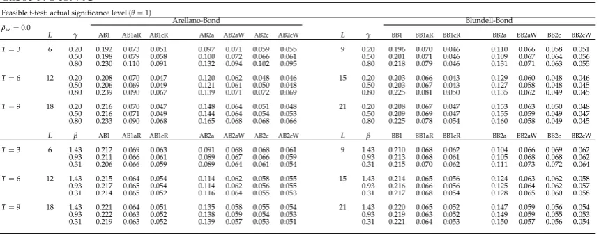
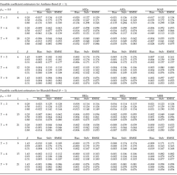
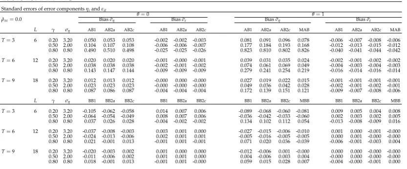
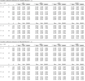
Abstract: Studies employing Arellano-Bond and Blundell-Bond GMM estimation for single linear dynamic panel data models are growing exponentially in number. However, for researchers it is hard to make a reasoned choice between many different possible implementations of these estimators and associated tests. By simulation the effects are examined of many options regarding: (i) reducing, extending or modifying the set of instruments; (ii) specifying the weighting matrix in relation to the type of heteroskedasticity; (iii) using (robustified) 1-step or (corrected) 2-step variance estimators; (iv) employing 1-step or 2-step residuals in Sargan-Hansen overall or incremental overidentification restrictions tests. This is all done for models in which some regressors may be either strictly exogenous, predetermined or endogenous. Surprisingly, particular asymptotically optimal and relatively robust weighting matrices are found to be superior in finite samples to ostensibly more appropriate versions. Most of the variants of tests for overidentification restrictions show serious deficiencies. A recently developed modification of GMM is found to have great potential when the cross-sectional heteroskedasticity is pronounced and the time-series dimension of the sample not too small. Finally all techniques are employed to actual data and lead to some profound insights.

Keywords: cross-sectional heteroskedasticity; model specification strategy; Sargan-Hansen (incremental) tests; variants of t-tests; weighting matrices; Windmeijer-correction

JEL:C12, C13, C15, C23, C26, C52, J22.

1. Introduction

One of the major attractions of analyzing panel data rather than single indexed variables is that they allow to cope with the empirically very relevant situation of unobserved heterogeneity correlated with included regressors. Econometric analysis of dynamic relationships on the basis of panel data, where the number of surveyed individuals is relatively large while covering just a few time periods, is very often based on GMM (generalized method of moments). Its reputation is built on its claimed flexibility, generality, ease of use, robustness and efficiency. Widely available standard software enables to estimate models including exogenous, predetermined and endogenous regressors consistently, while allowing for semiparametric approaches regarding the presence of heteroskedasticity and the type of distribution of the disturbances. This software also provides specification checks regarding the adequacy of the internal and external instrumental variables employed and the specific assumptions made regarding (absence of) serial correlation.

Popular are especially the GMM implementations put forward by Arellano and Bond [1].

instruments by adopting more orthogonality conditions. Extra orthogonality conditions can be based on certain homoskedasticity or stationarity assumptions or initial value conditions, see Blundell and Bond [2]. By abandoning weak instruments finite sample bias may be reduced, whereas by extending the instrument set with a few strong ones the bias may be further reduced and the efficiency enhanced. Presently, it is not clear yet how practitioners can best make use of these suggestions, because no set of preferred testing tools is yet available, nor a comprehensive sequential specification search strategy, which in a systematic fashion allow to select instruments by assessing both their validity and their strength, as well as to classify individual regressors accurately as relevant and either endogenous, predetermined or strictly exogenous. Therefore it happens often that in applied research models and techniques are selected simply on the basis of the perceived significance and plausibility of their coefficient estimates, whereas it is well known that imposing invalid coefficient restrictions and employing regressors wrongly as instruments will often lead to relatively small estimated standard errors. Then, however, these provide misleading information on the actual precision of the often seriously biased estimators.

The available studies on the performance of alternative inference techniques for dynamic panel data models have obvious limitations when it comes to advising practitioners on the most effective implementations of estimators and tests under general circumstances. As a rule, they do not consider various empirically relevant issues in conjunction, such as: (i) occurrence and the possible endogeneity of regressors additional to the lagged dependent variable, (ii) occurrence of individual effect (non-)stationarity of both the lagged dependent variable and other regressors, (iii) cross-section and/or time-series heteroskedasticity of the idiosyncratic disturbances, and (iv) variation in signal-to-noise ratios and in the relative prominence of individual effects. For example: the simulation results in Arellano and Bover [3], Hahn and Kuersteiner [4], Alvarez and Arellano [5], Hahn et al. [6], Kiviet [7], Kruiniger [8], Okui [9], Roodman [10], Hayakawa [11] and Han and Phillips [12] just concern the panel AR(1) model under homoskedasticity. Although an extra regressor is included in the simulation studies in Arellano and Bond [1], Kiviet [13], Bowsher [14], Hsiaoet al.[15], Bond and Windmeijer [16], Bun and Carree [1718], Bun and Kiviet [19], Gouriéroux

et al.[20], Hayakawa [21], Dhaene and Jochmans [22], Flannery and Hankins [23], Everaert [24] and Kripfganz and Schwarz [25], this regressor is (weakly-)exogenous and most experiments just concern homoskedastic disturbances and stationarity regarding the impact of individual effects. Blundell

et al. [26] and Bun and Sarafidis [27] include an endogenous regressor, but their design does not allow to control the degree of simultaneity; moreover, they stick to homoskedasticity. Harriset al.

[28] only examine the effects of neglected endogeneity. Heteroskedasticity is considered in a few simulation experiments in Arellano and Bond [1] in the model with an exogenous regressor, and just for the panel AR(1) case in Blundell and Bond [2]. Windmeijer [29] analyzes panel GMM with heteroskedasticity, but without including a lagged dependent variable in the model. Bun and Carree [30] and Juodis [31] examine effects of heteroskedasticity in the model with a lagged dependent and a strictly exogenous regressor under stationarity regarding the effects. Moral-Benito [32] examines stationary and nonstationary regressors in a dynamic model with heteroskedasticity, but the extra regressor is predetermined or strictly exogenous. Moreover, his study is restricted to time-series heteroskedasticity, while assuming cross-sectional homoskedasticity. In a micro context cross-sectional heteroskedasticity seems more realistic to us, whereas it is also trickier whenNis large andTsmall.

So, knowledge is still scarce with respect to the performance of GMM when it is not only needed to cope with genuine simultaneity (which we consider to be the core of econometrics), but also because of occurrence of heteroskedasticity of unknown form. Moreover, many of the simulation studies mentioned above did not systematically explore the effects of relevant nuisance

parameter values on the finite sample distortions to asymptotic approximations. We examine

on the validity of instruments worrying results have been obtained in Bowsher [14] and Roodman [10] for homoskedastic models. On the other hand Bun and Sarafidis [27] report reassuring results, but these just concern models whereT=3. Hence, it would be useful to examine more cases over an extended grid covering more dimensions. Our grid of examined cases will be much wider and have more dimensions. Moreover, we will deliberately explore both feasible and unfeasible versions of estimators and test statistics (in unfeasible versions particular nuisance parameter values are assumed to be known). Therefore we will be able to draw more useful conclusions on what aspects do have major effects on any inference inaccuracies in finite samples.

The data generating process designed here can be simulated for classes of models which may include individual and time effects, a lagged dependent variable regressor and another regressor which may be correlated with these and other individual effects and be either strictly exogenous or jointly dependent with regard to the idiosyncratic disturbances, whereas the latter may show a form of cross-section heteroskedasticity associated with both the individual effects. For a range of relevant parameter values we will verify in moderately large samples the properties of alternative GMM estimators, both 1-step and 2-step, focussing on alternative implementations regarding the weighting matrix and corresponding corrections to variance estimates according to the often practiced approach by Windmeijer [29]. This will include variants of the popular system estimator, which exploit as instruments the first-difference of lagged internal variables for the untransformed model in addition to lagged level internal variables as instruments for the model from which the individual effects have been removed. We will examine cases where the extra instruments are (in)valid in order to verify whether particular tests for overidentification restrictions have appropriate size and power, such that with reasonable probabilities valid instruments will be recognized as appropriate and invalid instruments will be detected and can be discarded. Moreover, following Kiviet and Feng [33], we shall investigate a rather novel modification of the traditional GMM implementation which aims at improving the strength of the exploited instruments in the presence of heteroskedasticity. Of course, also the simulation design used here has its limitations. It has only one extra regressor next to the lagged dependent variable, we only consider cross-sectional heteroskedasticity, and all basic random terms have been drawn from the normal distribution. Moreover, the design does not accommodate general forms of cross-sectional dependence between error terms. However, by including individual and time specific effects particular simple forms of cross-sectional dependence are accommodated.

The structure of this study is as follows. In Section 2 we first present the major issues regarding IV and GMM coefficient and variance estimation in linear models and on inference techniques on establishing instrument validity and regarding the coefficient values by standard and by corrected test statistics. Next in Section 3 the generic results of Section 2 are used to discuss in more detail than provided elsewhere the various options for their implementation in linear models for single dynamic simultaneous micro econometric panel data relationships with both individual and time effects and some form of cross-sectional heteroskedasticity. In Section 4 the Monte Carlo design is developed to analyze and compare the performance of alternative often asymptotically equivalent inference methods in finite samples of empirically relevant parametrizations. Section 5 summarizes the simulation results, from which some preferred techniques for use in finite samples of particular models emerge, plus a warning regarding particular types of models that require more refined methods yet to be developed. An empirical illustration, which involves data on labor supply earlier examined by Ziliak [34], can be found in Section 6, where we also formulate a tentative comprehensive specification search strategy for dynamic micro panel data models. Finally, in Section 7 the major findings are summarized.

2. Basic GMM results for linear models

general findings for linear regressions the examined implementations for specific linear dynamic panel data models follow easily in Section 3.

2.1. Model and estimators

Let the scalar dependent variable yi depend linearly on K regressors xi and an unobserved

disturbance termui, and let there beL≥Kvariableszi(the instruments) that establish orthogonality

conditions such that

yi=x0_iβ0+ui E[zi(yi−xi0β0)] =0

)

i=1, ...,n. (1)

Herexi and β0are K×1 vectors, β0containing the true values of the unknown coefficients, andzi

is anL×1 vector. Applying the analogy principle, the method of moments (MM) aims to find an estimator for model parameterβby solving theLsample moment equations

n−1Σ_in₌₁zi(yi−x0iβˆ) =0. (2)

Generally, these have a unique solution only whenL=Kand then yield ˆ

β= (Σn_i=1zixi0)−1Σin=1ziyi, (3)

provided the inverse exists. ForL > Kthe MM recipe to find a unique estimator is: minimize with respect toβthe criterion functionΣn_i=1[(yj−x0jβ)z0j]GΣiN=1[zi(yi−xi0β)]for some weighting matrixG.

It can be shown that the asymptotically optimal choice forGis an expression which has a probability limit that is proportional to the inverse of the asymptotic varianceVof n−1/2Σ_in₌₁ziui →d N(0,V).

Whenui ∼ iid(0,σu2)an optimal choice forGis proportional to the inverse ofΣni=1ziz0i and the MM

estimator is

ˆ

βIV= [X0Z(Z0Z)−1Z0X]−1X0Z(Z0Z)−1Z0y, (4)

where y = (y1· · ·yn)0, X = (x1· · ·xN)0 and Z = (z1· · ·zN)0. But, when E(ziui) = 0 while u =

(u1· · ·un)0 ∼ (0,σu2Ω), whereΩhas full rank and without loss of generalitytr(Ω) =n, the optimal

choice forGis a matrix proportional to(Z0ΩZ)−1_{, yielding MM estimator}

ˆ

βGMM = [X0Z(Z0ΩZ)−1Z0X]−1X0Z(Z0ΩZ)−1Z0y. (5)

Note that forΩ = Inthe latter formula simplifies to ˆβIV. WhenL =Kboth ˆβGMM and ˆβIVsimplify

to (3) or(Z0X)−1Z0y.

WhenΩis unknown and therefore (5) is unfeasible, one should use an informed guessΩ(0)to obtain the 1-step estimator ˆβ(_GMM1) , which is sub-optimal whenΩ(0)6=Ω, though consistent under the

assumptions made. Then the residuals

ˆ

u(1)=y−Xβˆ(_GMM1) (6)

are consistent for u, thus from them it should be possible to obtain an expression ˆΩ(1) such that plimn−1(Z0Ωˆ(1)Z−Z0ΩZ) =O. Substituting in (5) yields the 2-step estimator

ˆ

β(_GMM2) = [X0Z(Z0Ωˆ(1)Z)−1Z0X]−1X0Z(Z0Ωˆ(1)Z)−1Z0y, (7)

which is asymptotically equivalent to ˆβGMM and thus asymptotically optimal, given the L

2.2. Some algebraic peculiarities

It is well-known and easy to prove that all the above method of moment estimators are invariant to linear transformations of the matrix of instrumentsZ, as long as its rank is preserved.

DefiningPZ = Z(Z0Z)−1Z0 and ˆX = PZXone finds ˆβIV = (Xˆ0Xˆ)−1Xˆ0y, which highlights its

two-stage least-squares character. Now suppose thatX= (X1,X2)andZ = (Z1,Z2)withZ2 = X2

whereasXβ=X1β1+X2β2, whereβ1andβ2haveK1andK2elements respectively. Standard results

on partitioned regression yields

ˆ

β1,IV= (Xˆ10MXˆ2Xˆ1)

−1_Xˆ0

1MXˆ2y= (X

0

1PMX₂Z1X1)

−1_X0

1PMX₂Z1y, (8)

which is the IV estimator in the regression ofyon justX1using the L−K2instruments MX2Z1. This result is known as partialling out the predetermined regressorsX2. It follows from ˆX2=PZX2 =X2

which yields

MXˆ2Xˆ1=MX2PZX1=MX2(PX2+PMX₂Z1)X1=PMX₂Z1X1. A similar result is not straight-forwardly available for GMM because of the following.

Let positive definite matrixΩbe factorized as follows

Ω−1_=Ψ0_Ψ

, soΩ=Ψ−1(Ψ0)−1. (9)

Now define

y∗=Ψy, X∗=ΨX, Z†= (Ψ0)−1Z, (10) then

ˆ

βGMM = [X∗0Z†(Z†0Z†)−1Z†0X∗]−1X∗0Z†(Z†0Z†)−1Z†0y∗

= (X∗0P_Z†X∗)−1X∗0P_Z†y∗,

so GMM is equivalent to IV using transformed variables, but where Z has been transformed

differently. Therefore, ifX2is such thatX∗2 establishes valid instruments in the transformed model

y∗=X∗β+u∗, whereu∗∼(0,σ_u2In), the regressorsX2∗are not used as instruments in GMM in its IV

interpretation. They would, though, if one would deliberately chooseZ2=Ω−1X2.

As is well-known and easily verified, linear transformations of the matrix of instruments of the formZ=ZC, whereCis a full rankL×Lmatrix, have no effect on ˆβIVnor on ˆβGMM. However, there

is not such invariance when the matrixZis premultiplied by some transformation matrix, and hence not the columns but the rows ofZ are directly affected. It has been shown in Kiviet and Feng [33] that such transformations, chosen in correspondence with the required transformation of the model whenΩ 6= In, may lead to modified GMM estimation achieving higher efficiency levels and better

results in finite samples than standard GMM, provided the validity of the transformed instruments is maintained. We will examine here the effects of employing transformationZ∗=ΨZ, which provides the modified GMM estimator

ˆ

βMGMM= [X0Ω−1Z(Z0Ω−1Z)−1Z0Ω−1X]−1X0Ω−1Z(Z0Ω−1Z)−1Z0Ω−1y. (11)

When this can be made feasible, it yields ˆβ(_MGMM2) .

2.3. Particular test procedures

Inference on elements ofβ0based on ˆβ(_GMM2) of (7) requires an asymptotic approximation to its

distribution. Under correct specification the standard first-order approximation is

ˆ

It allows testing general restrictions by Wald-type tests. For an individual coefficient, sayβ0k=e0K,kβ0,

whereeK,kis aK×1 vector with all elements zero except itskthelement(1 ≤k≤K)which is unity,

testingH0:β0k=β0_kand allowing for one-sided alternatives, amounts to comparing test statistic W_βk= (e0_K,kβˆ(_GMM2) −β0_k)/{σˆ_u2e0_K,k[X0Z(Z0Ωˆ(1)Z)−1Z0X]−1eK,k}1/2 (13)

with the appropriate quantile of the standard normal distribution. Note that this test statistic is actually an asymptotic t-test; in finite samples the type I error probability may deviate from the chosen nominal level, also depending on whether ˆσu2 has been obtained from 1-step or from 2-step

residuals and any employed loss of degrees of freedom corrections. In fact it has been observed that the consistent estimator of the variance of two-step GMM estimatorsVard(βˆ

(2)

GMM)given in (12) often

underestimates the finite sample variance, because in its derivation the randomness of ˆΩ(1)is not taken into account. Windmeijer [29] provides a corrected formula [Varc(βˆ(_GMM2) ), see Appendix A,

which can be used in the corrected t-test

W_βc

k = (e

0

K,kβˆ

(2)

GMM−β0k)/{e

0

K,kVarc[(βˆ

(2)

GMM)eK,k}1/2. (14)

WhenL>Kthe overidentification restrictions can be tested by the Sargan-Hansen statistic

J_Z(1)=n(uˆ(1)0Z(Z0Ωˆ(1)Z)−1Z0uˆ(1))/(uˆ(1)0uˆ(1)), (15) which under correct specification and valid instruments Z is distributed as χ2_L−K asymptotically.

Because ˆΩ(1) is based on ˆu(1)_{, which relates to a consistent estimator, but not to an asymptotically}

optimal estimator, it might be better to perform at least one further iteration and use

J_Z(2)=n(uˆ(2)0Z(Z0Ωˆ(2)Z)−1Z0uˆ(2))/(uˆ(2)0uˆ(2)), (16) where ˆu(2) = y−Xβˆ(_GMM2) is used to construct ˆΩ(2). WhenZ = (Zm Za), where Zm is an n×Lm

matrix with Lm ≥ Kcontaining the instruments whose validity seems very likely, then, under the

maintained hypothesisE(Z0_mu) =0, one can test the validity of theL−Lmadditional instrumentsZa

by the incremental test statistic

J I_Z(2_a)=n[uˆ(2)0Z(Z0Ωˆ(2)Z)−1Z0uˆ(2)/(uˆ(2)0uˆ(2))−uˆ(m2)0Zm(Z0mΩˆm(2)Zm)−1Zm0 uˆ(m2)/(uˆ(2

)0

m uˆ(m2))], (17)

which under correct specification of the model with valid instruments Z is distributed as χ2_L−Lm

asymptotically. Of course, ˆu(m2)and ˆΩ(m2) are obtained by just using the instruments Zm. Note that

for m = K we have J I_Z(2_a) = J_Z(2) because in that case Z0muˆm(2) = 0. Hence, when m = K, explicit

specification of componentZmis meaningless.

In simulations it is interesting to examine as well unfeasible versions of the above test statistics, which exploit information that is usually not available in practice. This will produce evidence on what elements of the feasible asymptotic tests may cause any inaccuracies in finite samples. So, next to (13), (16) and (17) we will also examine

W_β(u)

k = (e

0

K,kβˆGMM−β0_k)/{σ_u2e_K0_,k[X0Z(Z0ΩZ)−1Z0X]−1eK,k}1/2, (18) J(_Zu)=uˆ0Z(Z0ΩZ)−1Z0uˆ/σu2, where ˆu=y−XβˆGMM, (19) J I(_Zu_a)= [uˆ0Z(Z0ΩZ)−1Z0uˆ−uˆ0mZm(Zm0 ΩZm)−1Zm0 uˆm]/σu2. (20)

3. Implementations for dynamic micro panel models

3.1. Model and assumptions

We consider the balanced linear dynamic panel data model(i=1, ...,N;t=1, ...,T)

yit=x0itβ+w0itγ+vit0δ+µ+τt+ηi+εit, (21)

wherexitcontainsKx≥0 strictly exogenous regressors (excluding a constant and fixed time effects), witareKw≥0 predetermined regressors (probably including lags of the dependent variable and other

variables affected by lagged feedback fromyitor just fromεit),vitareKv≥0 endogenous regressors

(affected by instantaneous feedback fromyitand therefore jointly dependent withyit),µis an overall

constant, theτt are random or fixed time effects, theηi are random individual specific effects (most

likely correlated with many of the regressors) such that

ηi∼iid(0,σ_η2), (22)

whereas

E(εit) =0, E(ε_it2) =σ_it2, E(εitεjs) =0, E(ηiεjt) =0, ∀i,j,t6=s. (23)

The parameter vector τ could have all its elements equal and then will be absorbed by the

overall interceptµof the model. However, it seems better to allow for time effects in addition to

an intercept, because this helps to underpin the assumption that both the idiosyncratic disturbances and the individual effects have expectation zero. Note, though, that for identification at least one restriction should be imposed on theT+1 scalar parameters represented byµandτ.

The classification of the regressors implies

E(xitεis) =0, E(witεi,t+l) =0, E(vitεi,t+1+l) =0, ∀i,t,s,l ≥0. (24)

For the sake of simplicity we assume that all regressors are time varying and that the vectorsxit,wit

orvit are defined fort = 1, ...,T. However, their elements may contain observations prior tot = 1

for regressors that are actually thelthorder lag of a current variable. Only these lagged regressors are observed fromt = 1−lonwards. This means that all regressors in (21), be it current variables or lags of them, have exactlyTobservations. So, any unbalancedness problems have been defined away; moreover, no internal instrumental variables can be constructed involving observations prior to those included inxi1,wi1orvi1.

Stacking theTtime-series observations of (21) the equation in levels can be written

yi=Xiβ+Wiγ+Viδ+ITτ+ιT(µ+ηi) +εi, (25)

whereyi = (yi1· · ·yiT)0,Xi= (xi1· · ·xiT)0,Wi = (wi1· · ·wiT)0,Vi= (vi1· · ·viT)0,τ= (τ1· · ·τT)0and ιTis theT×1 vector with all its elements equal to unity. We do allowKx = 0,Kw = 0,Kv =0, but

not all three at the same time, so

K=Kx+Kw+Kv>0. (26)

3.2. Removing individual effects by first differencing

First we consider estimating the model by GMM following the approach propounded by Arellano and Bond [1], see also Holtz-Eakinet al.[35]. To clarify this, and the consequences it may have for the time-dummies, we introduce the matrices

DT=



     

−1 1 0 · · · 0

0 −1 1 ...

..

. . .. ... 0

0 0 · · · −1 1



     

andD∗T−1=



     

1 0 0

−1 1 . .. ...

. .. 1 0 0 · · · −1 1



     

, (27)

whereDTis(T−1)×TandDT∗−1is its(T−1)×(T−1)submatrix after removing the first column.

By taking first differences the intercept and the individual effects are removed and one may estimate theNsets ofT−1 equationsDTyi =DTXiβ+DTWiγ+DTViδ+DTτ+DTεi. Denoting ˜yi =DTyi,

˜

Xi =DTXi, ˜Wi =DTWi, ˜Vi =DTVi, ˜εi=DTεiand ˜τ=DTτ, where ˜τt =τt−τt−1fort=2, ...,T, this

can compactly be expressed as ˜yi=R¯iα¯+ε˜i, where ¯Ri= (X˜i, ˜Wi, ˜Vi,IT−1)and ¯α= (β0,γ0,δ0, ˜τ0)0.

However, the popular Stata package xtabond2 reparametrizes the time-effects differently (as we found out by experimentation). It substitutes ˜τ =D∗_T−1τ∗. Hence,τ_t∗=τt−τ1fort=2, ...,T, and it

estimates

˜

yi=R˜iα˜+ε˜i, (28)

where ˜Ri= (X˜i, ˜Wi, ˜Vi,D∗T−1)and ˜α= (β0,γ0,δ0,τ∗0)0. So, basically, it addresses the problem that not

allTtime-dummy coefficients can be identified, by replacing the submatrix of regressorsDT, which

has rankT−1, by full rank matrixD∗_T−1, so by simply removing its first column, with the effect that coefficientsτ∗will be estimated.

Defining

QT= 0

0

IT−1

!

andAT=



    

1 0 · · · 0

1 1 0

..

. ... . .. ... 1 1 · · · 1



    

, (29)

whereQT isT×(T−1)and AT isT×Tlower-triangular, one easily finds thatDTQT = D∗T−1 =

A−_T−1₁. Instead ofτ∗, one can directly estimate ˜τ= D∗_T−1τ∗by xtabond2 by replacing in the equation

in levelsITτbyATτ∗∗, hence by replacing the time dummy variables by accumulated time dummies.

Here τ∗∗ = A−_T1τ = DT+1QT+1τ = DT+1(0,τ0)0 = (τ1, ˜τ0)0. Note thatDTAT = (0,IT−1). Hence,

IT−1τ˜ =τ˜would remain, after removal of the first column, as in ˜yi =R¯iα¯+ε˜i. Of course, many more

different transformations of theTcoefficientsτcan be estimated, though, by taking first differences

onlyT−1 linear transformations of them can be identified; by interpreting them appropriately no fundamental differences emerge.

To construct a full column rank matrix of instrumental variables Z = (Z0₁· · ·Z0_N)0, which expresses as many linearly independent orthogonality conditions as possible for (28), while restricting ourselves to internal variables,i.e.variables occurring in (21), we define the following vectors

xT_i0= (x_i0₁· · ·x0_iT), wt_i0= (w_i0₁· · ·w0_it), vt_i0 = (v0_i1· · ·v0_it). (30) Without making this explicit in the notation it should be understood that these three vectors only contain unique elements. Hence, if vectorxis(orwis)contains for 1 < s ≤ Ta particular value and

also its lag (which is not possible forvit), then this lag should be taken out since it already appears

inxi,s−1. MatrixZiis of order(T−1)×Land consists of four blocks (though some of these may be

void)

Zi = (Zix,Zwi ,Zvi,D

∗

The final block spans the same space asIT−1and could thus be replaced byIT−1. It is associated with

the fundamental moment conditionsE(˜εi) =0. Therefore, it could form part ofZieven if one imposes τ=0. For the other blocks we have

Z_ix=IT−1⊗xTi0, Ziw=



 

w1_i0 00 00

O . .. O

00 00 wT_i−10 

 , Z

v i =



    

00 00 00

v1_i0 00 00

O . .. O

00 00 vT_i−20 

    

. (32)

The maximum possible number of columns ofZ_ixisKxT(T−1), forZw_i it isKwT(T−1)/2 and forZ_iv

it isKv(T−1)(T−2)/2, thus

L≤(T−1){T[Kx+ (Kw+Kv)/2]−Kv+1}, (33)

whereas MM estimation requiresL≥K+T−1. It follows from (23) and (24) thatE(Z_i0ε˜i) =0 indeed.

In actual estimation one may use a subset of these instruments by taking the linear transformation

Z_i∗ = ZiC, whereCis anL×L∗matrix (with all its elements often being either zero, one or minus

one) of rank L∗ < L, providedL∗ ≥ K+T−1. In the above we have implicitly assumed that the variables are such thatZ= (Z0₁· · ·Z0_N)0will have full column rank, so another necessary condition is

N(T−1)≥L∗. Of course, it is not required that individual blocksZihave full column rank.

Despite its undesirable effect on the asymptotic variance of method of moments estimators, reducing the number of instruments may improve estimation precision, because it may at the same time mitigate estimation bias in finite samples, especially when weak instruments are being removed. So, instead of including the block D∗_T−1 or IT−1 in Zi one could – especially when the model has

no time-effects – replace it by IT−1ιT−1 = ιT−1. Regarding Zwi and Ziv two alternative instrument

reduction methods have been suggested, namely omitting long lags (see Bowsher14, Windmeijer29 and Bun and Kiviet19) and collapsing (see Roodman10, but also suggested in Anderson and Hsiao 36). Both are employed in Ziliak [34]; these two methods can also be combined.

Omitting long lags could be achieved by reducingZ_iwto, for instance, 

      

w0_i1 00 00 00 00 00 00

00 w0_i1 w0_i2 00 00 00 00

00 00 00 w0_i2 w0_i3 00 00

..

. ... ... O0 O0 . .. O0 O0

00 00 00 00 00 w_i0_,T−2 w0_i,T−1 

      

(34)

and similar forZv_i. The collapsed versions ofZ_iwand ofZ_ivcan be denoted as

Z∗_iw = 

     

w0_i1 00 · · · 00

w0_i2 w0_i1 ... ..

. . .. O

w0_i,T−1 w_i0_,T−2 · · · w0_i,1 

     

, Z_i∗v= 

       

00 00 · · · 00

v0_i1 00 00

v0_i2 v0_i1 ... ..

. . .. O

v0_i,T−2 w_i0_,T−3 · · · v0_i,1 

       

. (35)

Collapsing can be combined with omitting long lags, if one removes all the columns of Z_i∗w and

In corresponding ways, the column space ofZx_i can be reduced by including inZi either a limited

number of lags and leads, or the collapsed matrix

Z_i∗x= 

     

x0_i2 x_i0₁ 00 · · · 00

x0_i3 x_i0₂ x_i0₁ ... ..

. ... . .. O

x0_i,T x_i0_,T−1 x_i0_,T−2 · · · x0_i,1 

     

, (36)

or just its first two or three columns – or what is often done in practice – simply the difference between the first two columns, theKxregressors(∆xi2, ...,∆xiT)0.

It seems useful to distinguish the following specific forms of instrument matrix reduction of the case where all instruments associated with valid linear moment restrictions are being used. The latter case we label as A (all); the reductions are labelled C (standard collapsing), L0, L1, L2, L3 (which primarily restrict the lag length), and C0, C1, C2, C3 (which combine the two reduction principles). In all the reductions we replaceIT−1byιT−1when the model does not include time-effects. Regarding

Z_ix,Z_iw and Z_iv different types of reductions can be taken, which we will distinguish by using for example the characterization: Av, L2w, C1xetc. This leads to the particular reductions as indicated and defined in Table 1.

Table 1.Definition of labels for particular instrument matrix reductions

Ax :Zx_i Aw :Zw_i Av :Zv_i

L0x:diag(x0_i2, ...,x_iT0 ) L0w:diag(w0_i1, ...,w0_i,T−1) L0v:[0,diag(vi1, ...,vi,T−2)]0

L1x:diag(∆x0_i2, ...,∆x0_iT) L1w:diag(w0_i1,∆w0_i2, ...,∆w_i0_,T−1) L1v:[0,diag(vi1,∆vi2, ...,∆vi,T−2)]0

L2x:diag(x0_i1, ...,x0_i,T−1), L0x L2w:[0,diag(wi1, ...,wi,T−2)]0, L0w L2v:[0, 0,diag(vi1, ...,vi,T−3)]0, L0v

L3x:[0,diag(xi1, ...,xi,T−2)]0, L2x L3w:[0, 0,diag(wi1, ...,wi,T−3)]0, L2w L3v:[0, 0, 0,diag(vi1, ...,vi,T−4)]0, L2v

Cx :Z∗_ix Cw :Z∗_iw Cv :Z∗_iv

C0x_:(x

i2, ...,xiT)0 C0w:(wi1, ...,wi,T−1)0 C0v:(0,vi1, ...,vi,T−2)0

C1x_:(∆x

i2, ...,∆xiT)0 C1w:(0,∆wi2, ...,∆wi,T−1)0 C1v:(0, 0,∆vi2, ...,∆vi,T−2)0

C2x: C0x,(xi1, ...,xi,T−1)0 C2w: C0w,(0,wi1, ...,wi,T−2)0 C2v: C0v,(0, 0,vi1, ...,vi,T−3)0

C3x_{: C2}x_,(0,x

i1, ...,xi,T−2)0 C3w: C2w,(0, 0,wi1, ...,wi,T−3)0 C3v: C2v,(0, 0, 0,vi1, ...,vi,T−4)0

Note that for all three types of regressors L2, like L1, uses one extra lag compared to L0, but does not impose the first-difference restrictions characterizing L1. We skipped a similar intermediary case between L2 and L3. Self-evidently L2xcan also be represented by combining diag(x_i0₁, ...,x0_i,T−1) with L1x, and similar for L2w and L2v. The reductions C0 and C1, which yield just one instrument per regressor, constitute generalizations of the classic instruments suggested by Anderson and Hsiao [36]. These may lead to just identified models where the number of instruments equals the number of regressors which provokes the non-existence of moments problem. To avoid that, and also because we suppose that in general some degree of overidentification will have advantages regarding both estimation precision and the opportunity to test model adequacy, one may choose to restrict oneself to the popular C1xand the reductions C and C3 as far as collapsing is concerned. In C3 just the first three columns of the matrices in (35) and (36) are being used as instruments.

3.2.1. Alternative weighting matrices

We assumed in (23) that the εit are serially and cross-sectionally uncorrelated but may be

heteroskedastic. Let us define the matrixΩi = diag(σ_i2₁, ...,σ_iT2), thusεi ∼ (0,Ωi)and ˜εi = DTεi ∼

(0,DTΩiD0T). Under standard regularity we have

N−1/2ΣN_i=1Z_i0ε˜i d

Hence, the optimal GMM estimator of ˜αof (28) should use a weighting matrix such that its inverse has

probability limit proportional to plimN−1ΣN_i=1Z_i0DTΩiD0TZi. This can be achieved by first obtaining

a consistent 1-step GMM estimator

b˜

α(1)= [(ΣN_i=1R˜0_iZi)G(0)(ΣiN=1Z0iR˜i)]−1(ΣiN=1R˜0iZi)G(0)(ΣNi=1Zi0y˜i), (38)

which uses the weighting matrix

G(0)=ΣN_i=1Z0_iDTD0TZi

−1

. (39)

This is already efficient ifΩi = σ_ε2IT; otherwise, in a second step, the consistent 1-step residuals

bε˜

(1)

i =y˜i−R˜ibα˜

(1)

can be used to construct the asymptotically optimal weighting matrix

ˆ

G(a1)= (ΣiN=1Zi0bε˜

(1)

i bε˜

(1)0

i Zi)−1. (40)

An alternative is using

ˆ

G_b(1)= (Σ_iN₌₁Z_i0Hˆ_i(1)bZi)−1, (41)

where ˆH_i(1)bis the band matrix

ˆ

H_i(1)b = 

           

bε˜

(1)

i2 bε˜

(1)

i2 bε˜

(1)

i2bε˜

(1)

i3 0 · · · 0

bε˜

(1)

i3 bε˜

(1)

i2 bε˜

(1)

i3bε˜

(1)

i3 bε˜

(1)

i3bε˜

(1)

i4 0

0 bε˜

(1)

i4bε˜

(1)

i3 bε˜

(1)

i4bε˜

(1)

i4 . .. 0

..

. . .. . .. . .. ...

0 . .. bε˜

(1)

i,T−1bε˜

(1)

i,T−1 bε˜

(1)

i,T−1bε˜

(1)

iT

0 0 0 · · · bε˜

(1)

iTbε˜

(1)

i,T−1 bε˜

(1)

iTbε˜

(1)

iT



           

. (42)

Both(NGˆa(1))−1and (NGˆb(1))−1 have a probability limit equal to the limiting variance of (37). The

latter is less robust, but may converge faster whenΩiis diagonal indeed. On the other hand (41) may

not be positive definite, whereas (40) is.

For the special case Ωi = σ_ε2_,iIT of cross-section heteroskedasticity but time-series

homoskedasticity, one could use ˆ

G(c1)= (ΣNi=1Zi0Hˆ

(1)c

i Zi)−1, (43)

with

ˆ

H_i(1)c=σˆ_ε2,_,i(1)H=σˆ_ε2,_,i(1) 

        

2 −1 0 · · · 0

−1 2 . .. ... ...

0 . .. ... ... 0

..

. . .. ... 2 −1

0 · · · 0 −1 2



        

, (44)

whereH=DTD0Tand

ˆ

σ_ε2,_,i(1)=b˜ε

(1)0

i H

−1

bε˜

(1)

i /(T−1). (45)

Of course, these N estimators are not consistent for T finite. However, a consistent estimator for

σ_ε2= N−1Σ_iN₌₁σ_ε2_,iis given by

ˆ

The three different weighting matrices can be used to calculate alternativebα˜

(2)

(j) estimators for

j∈ {a,b,c}according to

b˜

α(₍2_j))= [(ΣN_i=1R˜0_iZi)Gˆ

(1)

j (Σ N

i=1Z0iR˜i)]−1(ΣiN=1R˜0iZi)Gˆ

(1)

j (Σ N

i=1Zi0y˜i). (47)

When the employed weighting matrix is asymptotically optimal indeed, the first-order asymptotic approximation to the variance of bα˜

(2)

(j) is given by the inverse of the matrix in square brackets.

From this (corrected) t-tests are easily obtained, see Section 3.4. Matching implementations of Sargan-Hansen statistics follow easily too, see Section 3.5. Note that estimators for σ_ε2_,i or σ_ε2 can

also be obtained by employing second-stage residuals.

Let bα˜ represent any of the consistent estimators of ˜α mentioned above, and consider the residuals ˆu†_i = yi−(Xi,Wi,Vi,QT)bα˜. From these we find µ\+τ1 = N−1T−1ΣiN=1ι0Tuˆi†, giving ˆui =

ˆ

u†

i −µ\+τ1, which forN →∞converges toui = ιTηi+εi. SinceE(uiu0i) = σε2,iIT+σ

2

ηιTι

0

Twe have

plimN−1Σ_iN₌₁uˆiuˆ0i = σε2IT+σ

2

ηιTι

0

T. This yields plimN−1ΣiN=1ι 0

Tuˆiuˆ0iιT = Tσε2+σ

2

ηT

2_{from which the}

consistent estimatorT−2N−1Σ_iN₌₁(ι0_Tuˆi)2−T−1σˆε2,(1)forση2follows. From simulations we established that, especially when ση is relatively small, this estimator is often negative. An alternative more satisfactory consistent estimator turns out to be

ˆ

ση2,(1)=T

−1_N−1_ΣN

i=1uˆ0iuˆi−σˆε2,(1). (48) This does not hinge as much on the serial uncorrelatedness of theεit. However, estimator (48) can be

negative too, especially whenση/σεis small orTis very small. When this happens it seems reasonable to set ˆση2,(1) = 0. Note that this does not jeopardize the consistency of the estimator; therefore we followed this approach in the simulations, rather then using the non-negative estimatorN−1Σ_iN₌₁ηˆ_i2, where ˆηi=T−1ΣTt=1uˆ†it−µ\+τ1, since this is inconsistent, becauseE(ηˆi2)6=ση2.

3.3. Respecting the equation in levels as well

In this subsection we will examine whether the first-difference operation in the foregoing subsection implied a loss of valid orthogonality conditions embodied by our initial assumptions made in subsection 3.1.

Sinceτ=τ1ιT+QTτ∗, we can rewrite model (25) as

yi =Xiβ+Wiγ+Viδ+QTτ∗+ (µ+τ1+ηi)ιT+εi

=Riα˜+ (µ+τ1)ιT+ui

=R∗_iα¨+ui, (49)

whereRi = (Xi,Wi,Vi,QT),R∗i = (Ri,ιT)and (K+T)×1 vector ¨α = (˜α0,µ+τ1)0; note that ˜Ri = DTRi.

RegressorιTis a valid instrument for model (49). It embodies the single orthogonality condition E[ΣT_t=1(ηi+εit)] = E[ΣTt=1uit] = 0 (∀i), which is implied by theT+1 assumptionsE(ηi) = 0 and E(εit) = 0 (fort = 1, ...,T)made in (22) and (23). TheseT+1 assumptions can also be represented

(through linear transformation) by (i)E(ηi) =0, (ii)E(∆εit) =0 (fort=2, ...,T)and (iii)E(ΣTt=1uit) =

0. Because we cannot express ηi exclusively in observed variables and unknown parameters it is

impossible to convert (i) into a separate sample orthogonality condition. The T−1 orthogonality conditions (ii) are already employed by Arellano-Bond estimation, through including IT−1orD∗T−1

inZi of (31) for the equation in first differences. Orthogonality condition (iii), which is in terms of

the level disturbance, can be exploited by including the columnιTin thei-th block of an instrument

Combining theT−1 difference equations and theTlevel equations in a system yields ¨

yi=R¨iα¨+u¨i, (50)

for each individuali, where ¨yi = (y˜i0,y0i)0, ¨Ri = (R˜∗0i ,R∗0i )0, with ˜R∗i = (R˜i, 0), so it is extended by

an extra column of zeros (to annihilate coefficient µ+τ1 in the equation in first differences), and

¨

ui = (˜ε0_i,u0_i)0. We find that E(˜εiu0i) = E(Dεiε0_i) = DΩi and E(uiu0i) = E[(ηiιT+εi)(ηiιT+εi)0] = σ_η2ιTι0_T+Ωi, so

E(u¨iu¨0i) =

DΩiD0 DΩi ΩiD0 Ωi+σ_η2ιTι0_T

!

. (51)

Model (50) can be estimated by MM using theN(2T−1)×(L+1)matrix of instruments with blocks

¨

Zi = Zi 0 O ιT

!

, (52)

providedN(2T−1)≥L+1≥K+T. Since both ¨Riand ¨Zicontain a column(00,ι0_T)0, and due to the

occurrence of theO-block in ¨Zi, by a minor generalization of result (8) the IV estimator of ¨αobtained

by using instrument blocks ¨Ziin (50) will be equivalent regarding ˜αwith the IV estimator of equation

(28) using instruments with blocks Zi. That the same holds here for GMM under cross-sectional

heteroskedasticity when using optimal instruments is due to the very special shape of ¨Zi and is

proved in Appendix B. Hence, there seems no good reason to estimate the system, just in order to exploit the extra valid instrument(00,ι0_T)0.

3.3.1. Effect stationarity

However, more valid internal instruments can be found for the equation in levels when some of the regressorsXi,Wi orVi are known to be uncorrelated (likeιT) with the individual effects, or

(which is more general) have time-invariant correlation with the individual effects. Then, after first differencing, these explanatory variables will be uncorrelated withηi. Letrit = (x

0

it,w

0

it,v

0

it)0contain

theK = Kx +Kw+Kv unique elements ofrit which are effect stationary, by which we mean that E(ritηi)is time-invariant, so that

E(∆r_itηi) =0, ∀i, t=2, ...,T.

This implies that for the equation in levels the orthogonality conditions

E[∆x_it(ηi+εis)] =0 E[∆w_it(ηi+εi,t+l)] =0 E[∆v_it(ηi+εi,t+1+l)] =0

  

 

∀i,t>1,s≥1,l≥0 (53)

hold. Whenw_itincludesyi,t−1, then apparentlyyitis effect stationary so that the adopted model (21)

suggests that all regressors inritmust be effect stationary, resulting inK=K.

Like for the T −1 conditions E(∆ε_it) = 0 discussed below equation (49), many of the conditions (53) are already implied by the orthogonality conditions E(Z_i0ε˜i) = 0 for the equation

in first-differences. In Appendix C we demonstrate that a matrix ˜Z_isof instruments can be designed for the equation in levels (49) just containing instruments additional to those already exploited by

E(Z_i0ε˜i) =0, whilstE[Z˜is0(ηiιT+εi)] =0. This is theT×Lmatrix

˜

whereL=K(T−1)−Kv +1, with

˜

Z_ix= 

      

00 00 · · · 00

∆x0

i2 00 · · · 00

00 ∆x_i30 00

..

. . ..

00 00 ∆x_iT0



      

, ˜Z_iw= 

      

00 00 · · · 00

∆w0

i2 00 · · · 00

00 ∆w_i30 00

..

. . ..

00 00 ∆w_iT0



       ,

˜

Z_iv= 

      

00 · · · 00 00 · · · 00

∆v0

i2 0

0

. ..

00 ∆v_i,T0₋₁ 

       .

Under effect stationarity of the K _{variables (53) the system (50) can be estimated while}

exploiting the matrix of instruments

¨

Zs_i = Zi O

O Z˜s_i !

. (55)

If one decides to collapse the instruments included inZi, it seems reasonable to collapse ˜Zsi as well

and replace it by

¨

Z∗_is = 

      

00 00 00 1

∆x0

i2 ∆w 0

i2 00 1

∆x0

i3 ∆w 0

i3 ∆v 0

i2 1

..

. ... ... ...

∆x0

iT ∆w

0

iT ∆v

0

i,T−1 1



      

. (56)

Note that ¨Z_i∗shasL=K+1 columns.

3.3.2. Alternative weighting matrices under effect stationarity

For the above system we have

N−1/2ΣN_i=1Z¨s 0

i u¨i d

→N(0, plimN−1ΣN_i=1Φi), (57)

with

Φi=

Z_i0DΩiD0Zi Zi0DΩiZ˜si

˜

Zs0

i ΩiD0Zi Z˜is0(Ωi+σ_η2ιTι0_T)Z˜s_i !

. (58)

Hence a feasible initial weighting matrix is given by

S(0)(q) = [ΣN_i=1Φ(_i0)(q)]−1, (59) where

Φ(0)

i (q) =

Z_i0DD0Zi Zi0DZ˜si

˜

Z_is0D0Zi Z˜is0(IT+qιTι0_T)Z˜s_i !

withqsome nonnegative real value. Weighting matrixS(0)(q)would be optimal ifΩi = σ_ε2IT with q=σ_η2/σ_ε2. For any nonnegativeqa consistent 1-step GMM system estimator is given by

b¨

α(1)(q) = [(ΣN_i=1R¨0_iZ¨_is)S(0)(q)(Σ_iN₌₁Z¨_is0R¨i)]−1(ΣiN=1R¨ 0

iZ¨si)S(0)(q)(ΣNi=1Z¨s 0

i y¨i). (60)

Next, in a second step, the consistent 1-step residuals bu¨

(1)

i = y¨i−R¨ibα¨

(1)

(q) can be used to construct the asymptotically optimal weighting matrix

ˆ

S(a1)= (ΣiN=1Z¨is0bu¨

(1)

i bu¨

(1)0

i Z¨is)−1, (61)

wherebu¨

(1)

i = (bε˜

s(1)0

i , ˆu s(1)0

i )0 withb˜ε

s(1)

i =y˜i−R˜∗ibα¨

(1)

(q)and ˆus_i(1)= yi−R∗ibα¨

(1)

(q). However, several alternatives are possible. Consider weighting matrix

ˆ

S(_b1)= "

ΣN i=1

Z_i0Hˆ_is(1)Zi Zi0Dˆ s(1)

i Z˜si

˜

Z_is0Dˆ_is(1)0Zi Z˜is0uˆ s(1)

i uˆ s(1)0

i Z˜si

!#−1

, (62)

where ˆH_is(1)is self-evidently like ˆH_i(1)bbut on the basis of the residualsbε˜

s(1)

i , and

ˆ

D_is(1)=             

bε˜

s(1)

i2 uˆ

s(1)

i1 b˜ε

s(1)

i2 uˆ

s(1)

i2 0 · · · 0 0

0 b˜ε

s(1)

i3 uˆ

s(1)

i2 bε˜

s(1)

i3 uˆ

s(1)

i3 0

..

. . .. . .. . .. ...

..

. . .. . .. ... ...

0 . .. bε˜

s(1)

i,T−1uˆ

s(1)

i,T−1 b˜ε

s(1)

i,T−1uˆ

s(1)

iT

0 0 0 · · · 0 b˜ε

s(1)

iT uˆ s(1)

iT              . (63)

For the special caseσ_ε2Ωi=σ_ε2_,iITof cross-section heteroskedasticity and time-series homoskedasticity

one can use the weighting matrix

ˆ

S(c1)=

" ΣN

i=1σˆ 2,s(1)

ε,i

Z_i0HZi Z0iDZ˜is

˜

Z_is0D0Zi Z˜si0[IT+ (σˆ

2,(1)

η / ˆσ

2,s(1)

ε,i )ιTι

0

T]Z˜is

!#−1

, (64)

where

ˆ

σ_ε2,_,is(1)=bε˜

s(1)0

i H

−1

bε˜

s(1)

i /(T−1), (65)

ˆ

σ_η2,s(1)=T−1N−1Σ_iN₌₁uˆs_i(1)0uˆs_i(1)−N−1ΣN_i=1σˆ_ε2,_,is(1). (66)

Forj∈ {a,b,c}three alternative 2-step system estimators

b¨

α₍(2_j))= [(ΣN_i=1R¨_i0Z¨_is)Sˆ(_j1)(Σ_iN₌₁Z¨s_i0R¨i)]−1(ΣNi=1R¨ 0

iZ¨is)Sˆ

(1)

j (ΣiN=1Z¨s 0

i y¨i) (67)

are obtained, where the inverse matrix expression can be used again to estimate the variance ofbα¨

(2) (j)

if all employed moment conditions are valid.

3.4. Coefficient restriction tests

combination with a robust variance estimate (which takes possible heteroskedasticity into account). The 2-step estimators can be used in combination with the standard or a corrected variance estimate.1

When testing particular coefficient values, the relevant element of estimatorbα˜

(1)

given in (38) should under homoskedasticity be scaled by the corresponding diagonal element of the standard expression for its estimated variance given by

d Var(bα˜

(1)

) =N−1Σ_iN₌₁σˆ_ε2,_,i(1)Ψ, withΨ= [(ΣN_i=1R˜0_iZi)G(0)(ΣiN=1Z0iR˜i)]−1, (68)

where ˆσ_ε2,_,i(1)is given in (45). Its robust version under cross-sectional heteroskedasticity uses forj ∈

{a,b,c}

d Var_(j)(bα˜

(1)

) =Ψ(Σ_iN₌₁R˜0_iZi)G(0)[Gˆ(j1)]

−1_G(0)_(ΣN

i=1Zi0R˜i)Ψ. (69)

However, under heteroskedasticity the estimatorsbα˜

(2)

(j) given in (67) are more efficient. The standard

estimator for their variance is

d Var(bα˜

(2)

(j)) = [(ΣNi=1R˜ 0

iZi)Gˆ_j(1)(ΣNi=1Z 0

iR˜i)]−1. (70)

The corrected version[Varc(bα˜

(2)

(j))requires derivation fork=1, ...,K−1 of the actual implementation

of matrix∂Ω(β)/∂β_k of Appendix A which is here N(T−1)×N(T−1). We denote itsi-th block

as∂Ω˜(j)i(α˜)/∂α˜k. For the a-type weighting matrix2the relevantT−1×T−1 matrix∂ε˜iε˜0_i/∂α˜k with

˜

εi =y˜i−R˜iα˜, is−(˜εiR˜0ik+R˜ikε˜0_i), where ˜Rikdenotes thek-th column of ˜Ri. For weighting matrix b it

simplifies to the matrix consisting of the main diagonal and the two first sub-diagonals of−(ε˜iR˜0_ik+

˜

Rikε˜0_i)with all other elements zero. And∂Ω˜(c)i(˜α)/∂α˜k=−2[ε˜0_iH−1R˜ik/(T−1)]H. So, we find

[ Varc(bα˜

(2)

(j)) =Vard(bα˜

(2)

(j)) +Fˆ(j)Vard(bα˜

(2)

(j)) +Vard(bα˜

(2)

(j))Fˆ(j)+Fˆ(j)Vard_(j)(bα˜

(1)

)Fˆ₍0_j), (71) with thek-th column of ˆF(j)given by

ˆ

F_(j)·k=−Vard(bα˜

(2)

(j))(ΣNi=1R˜ 0

iZi)Gˆj(1) ΣNi=1Z 0

i

∂Ω˜_(j)i(α˜) ∂α˜k

b˜

α(1)

Zi

! ˆ

G_j(1)(Σ_iN₌₁Z_i0bε˜

(2)

i ). (72)

All above expressions become a bit more complex when considering Blundell-Bond estimation of theKcoefficients ¨α. The suboptimal 1-step estimator (60) of ¨αshould not be used for testing, unless

in combination with

d Var(bα¨

(1)

) =Φ(ΣN_i=1R¨0_iZ¨_is)S(0)(q)[S(0)(σˆ_η2,s(1)/ ˆσ_ε2,s(1))]−1S(0)(q)(Σ_iN₌₁Z¨_is0R¨i)Φ, (73)

under homoskedasticity, or a robust variance estimator, which is

d Var_(j)(bα¨

(1)

) =Φ(Σ_iN₌₁R¨0_iZ¨_is)S(0)(q)[Sˆ(_j1)]−1S(0)(q)(ΣN_i=1Z¨_is0R¨i)Φ, (74)

whereΦ = [(ΣN_i=1R¨0_iZ¨_is)S(0)(q)(Σ_iN₌₁Z¨_is0R¨i)]−1. It seems better of course to use the efficient estimator

b¨

α(₍2_j))of (67). The standard expression for its estimated variance is

d Var(bα¨

(2) (j)) = [(Σ

N

i=1R¨0iZ¨is)Sˆ

(1)

j (Σ N

i=1Z¨si0R¨i)]−1. (75)

Their corrected versions can be obtained by a formula similar to (71) upon changing ˜αin ¨αand ˆF(j)·k

of (72) in

ˆ

F(j)·k=−Vard(bα¨

(2) (j))(Σ

N

i=1R¨0iZ¨si)Sˆ

(1)

j Σ N i=1Z¨si0

∂Ω¨_(j)i(α¨) ∂α¨k

b¨

α(1) ¨

Z_is !

ˆ

S(_j1)(Σ_iN₌₁Z¨_is0bε¨

(2)

i ), (76)

where the block of∂Ω¨_(j)i(α¨)/∂α¨kcorresponding to the equation in first differences is similar as before,

but with an extra column and row of zeros for the intercept. The block corresponding to the equation in levels we took for weighting matrices a and b equal to∂uiu0i/∂α¨k=−(uiR¯∗0ik+R¯ik∗u0i), and for type

c

∂{ε˜0_iH−1ε˜i/(T−1) +ΣiN=1[(ι0Tui)2−u0iui]/[NT(T−1)]}IT/∂α¨k,

for which the first term yields−2[(˜ε0_iH−1R˜ik)/(T−1)]IT, and the second gives

−2{ΣN

i=1(ι0TuiR¯∗0ikιT−R¯∗0ikui)/[NT(T−1)]}IT.

For the nondiagonal upperblock of∂Ω¨_(j)i(¨α)/∂α¨k we took in cases a and b∂ε˜iu0i/∂α˜k = −(˜εiR¯∗0ik+

˜

Riku0i)and for the derivative with respect to the intercept−ε˜iι0_T. In case c it is−2[(˜ε0_iH−1R˜ik)/(T−

1)]Dand a zero matrix for the derivative with respect to the intercept.

3.5. Tests of overidentification restrictions

Using Arellano-Bond and Blundell-Bond type estimation, many options exist with respect to testing the overidentification restrictions. These options differ in the residuals and weighting matrices being employed. After 1-step Arellano-Bond estimation, see (38) and (45), we have test statistic

J AB(1,0)= (ΣN_i=1bε˜

(1)0

i Zi)(ΣiN=1Z0iHZi)−1(ΣiN=1Z0ib˜ε

(1)

i )/(N−1ΣiN=1σˆ 2,(1)

i ), (77)

which is only valid in case of homoskedasticity. Alternatively, after 1-step estimation the

heteroskedasticity-robust test statistics

J AB(_j1,1)= (Σ_iN₌₁bε˜

(1)0

i Zi)Gˆ(j1)(ΣNi=1Zi0bε˜

(1)

i ), j∈ {a,b,c} (78)

may be used, where ˆG(_j1)is given in (40), (41) and (43). From (67) one may obtain 2-step residualsbε˜

(2)

i(j) =y˜i−R˜∗ibα¨

(2)

(j), and from these overidentification

restrictions test statistics can be calculated too, which may differ depending on whether the j-th weighting matrix is now obtained still from 1-step or already from 2-step residuals. This leads to

J AB(_j2,h)= (ΣN_i=1bε˜

(2)0

a,i Zi)Gˆ(jh)(ΣiN=1Z0ibε˜

(2)

a,i), forh∈ {1, 2} (79)

where the 2-step weighting matrices are either Gˆ(a2) = (ΣiN=1Z0ib˜ε

(2)

i(a)bε˜

(2)0

i(a)Zi)−1, Gˆb(2) =

(ΣN_i=1Z_i0Hˆ_i(2)bZi)−1or ˆG(c2) = (Σ_iN₌₁σˆ2,(2)

ε,i(c)Z 0

iHZi)−1, and ˆH_i(2)bis like ˆH_i(1)b of (42), though usingbε˜

(2)

i(b)

instead ofbε˜

(1)

i ; furthermore ˆσ

2,(2)

ε,i(c)=bε˜

(2)0

i(c)H−1bε˜

(2)

i(c)/(T−1).

Exploiting effect stationarity of a subset of the regressors by estimating the Blundell-Bond system leads to the 1-step test statistics

JBB(1,0)= (ΣN_i=1bu¨

(1)0

i Z¨si)S(0)(σˆ

2,s(1)

η / ˆσ

2,s(1)

ε )(Σ

N i=1Z¨s

0

i bu¨

(1)

i )/ ˆσ

2,s(1)

ε , (80)

JBB(_j1,1)= (ΣN_i=1bu¨

(1)0

i Z¨si)Sˆ

(1)

j (Σ N i=1Z¨s

0

i bu¨

(1)

where ˆσε2,s(1) = ΣNi=1σˆ 2,s(1)

ε,i /NandS

(0)_{(·)and ˆS}(1)

j can be found in (59), (61), (62) and (64). Defining

the various 2-step residuals and variance estimators asbu¨

(2)

i(j) =y¨i−R¨ibα¨

(2) (j) = (bε˜

s(2)0

i(j) , ˆu

s(2)0

i(j) ) 0 _{and ˆ}

σ_ε2,_,is₍(_j2₎)

and ˆσ2,(2)

η(j) similar to (65) and (66) though obtained from the appropriate two-step residualsbε˜

s(2)

i(j) =

˜

yi−R˜∗ibα¨

(2) (j) and ˆu

s(2)

i(j) =yi−R ∗

ibα¨

(2)

(j), the statistics to be used after 2-step estimation are

JBB(_j2,h)= (Σ_iN₌₁ub¨

(2)0

i(j)Z¨is)Sˆ

(h)

j (ΣiN=1Z¨si0bu¨

(2)

i(j)), (82)

where ˆS(a2) and ˆS(b2)are like ˆS

(1)

a and ˆS(b1), except that they use bu¨

(2)

i(a) andbu¨

(2)

i(b)instead of bu¨

(1)

i . With

respect to ˆS(c2)one can use

ˆ

S(c2)=

" ΣN

i=1σˆ 2,s(2)

ε,i(j)

Z_i0HZi Z0iDZ˜is

˜

Zs0

i D0Zi Z˜si0[IT+ (σˆ2,(2)

η(c)/ ˆσ

2,s(2)

ε,i(c))ιTι

0

T]Z˜is

!#−1 .

Under their respective null hypotheses the tests based on Arellano-Bond estimation follow asymptoticallyχ2distributions withL−K−T+1 degrees of freedom, whereas the tests based on

Blundell-Bond estimates haveL+L−K−Tdegrees of freedom3. Self-evidently tests on the effect stationarity related orthogonality conditions are given by

JES(1,0)=JBB(1,0)−J AB(1,0), (83)

JES_j(l,h)=JBB(_jl,h)−J AB_j(l,h), 0<l≤h∈ {1, 2}, j∈ {a,b,c} (84) and should be compared with aχ2critical value forL−1 degrees of freedom.4

3.6. Modified GMM

In the special case that panel model (25) has cross-sectional heteroskedasticity and no time-series heteroskedasticity, hence

σ_ε2Ωi =σ_ε2_,iIT, withΣiN=1σε2,i=σ

2

εN, (85)

we can easily employ MGMM estimator (11). However, because H−1 is not a lower-triangular

matrix, not all instruments σ_ε−_,i2H−1Zi would be valid for the equation in first-differences. This

problem can be avoided by using, instead of first-differencing, the forward orthogonal deviation (FOD) transformation for removing the individual effects. Let

B= 

       

T−1

T 0 0 · · · 0

0 T_T−₋2₁ 0 · · · 0 ..

. 0 . .. ... ...

..

. ... . .. 2₃ 0

0 0 · · · 0 1₂



       

1/2

       

1 − 1

T−1 · · · −T−11 −T−11

0 1 − 1

T−2 · · · −T−12 −T−12

..

. ... . .. . .. ... ...

0 0 . .. 1 −1

2 −12

0 0 · · · 0 1 −1



       

, (86)

3 _{Package xtabond2 for Stata always reportsJ AB}(1,0)_{after Arellano-Bond estimation, which is inappropriate when there}

is heteroskedasticity. After requesting for robust standard errors in 1-step estimation it presents alsoJ AB(a2,1)instead of

J AB(a1,1). Requesting 2-step estimation also presents bothJ AB(1,0)andJ AB

(2,1)

a . Blundell-Bond estimation yieldsJBB(1,0) andJBB(2,1)

, although a version ofJBB(1,0)

is reported that does not use weighting matrixS(0)_(ˆ

ση2,s(1)/ ˆσ 2,s(1) ε ), butS

(0)₍

0), which is only valid under homoskedasticity andσ_η2=0. Package xtabond2 addresses overidentification tests after 1-step

estimation always as "Sargan test" and after 2-step estimation as "Hansen test".

4 _{By specifying instruments in separate groups, xtabond2 presents for each separate group the corresponding incrementalJ}

and ˇεi= Bεi. ThenBιT =0 andBui =εˇi ∼(0,σ_ε2_,iIT−1)provided (85) holds, whereasE(Z_i0εˇi) =0 for Zigiven by (31). Hence, premultiplying modelyi=Riα˜+ (µ+τ1+ηi)ιT+εibyByields

ˇ

yi=Rˇiα˜+εˇi, (87)

where ˇyi = Byi and ˇRi = BRi. Estimating this by GMM, but using an instrument matrix

with componentsσ_ε−_,i2Zi, yields the unfeasible MABu estimator for the model with cross-sectional

heteroskedasticity, which is

b˜

αMABu= [(ΣiN=1σε−,i2Rˇ

0

iZi)(ΣNi=1σε−,i2Z

0

iZi)−1(ΣiN=1σε−,i2Z

0

iRˇi)]−1×

(ΣN_i=1σ_ε−_,i2Rˇ_i0Zi)(ΣiN=1σε−,i2Z

0

iZi)−1(ΣiN=1σε−,i2Z

0

iyˇi). (88)

Note that the exploited moment conditions are hereE(σ_ε−_,i2Z_i0εˇi) =σ_ε−_,i2E(Z0_iεˇi) =0. Forσ_ε2_,i >0 these

are intrinsically equivalent withE(Z_i0εˇi) =0, but they induce the use of a different set of instruments

yielding a different estimator. That it is most likely that the unfeasible standard AB estimator ABu, which uses instrumentsσ_ε,iZi for regressorsσ_ε−_,i1Rˇi, will generally exploit weaker instruments than

MABu, which usesσ_ε−_,i1Zifor regressorsσ_ε−_,i1Rˇi, should be intuitively obvious.

To convert this into a feasible procedure, one could initially assume that all σ_ε2_,i are equal.

Then the first-step MGMM estimatorbα˜

(1)

MAB is numerically equivalent to AB1 of (38), provided all

instruments are being used.5Next, exploiting (45), the feasible 2-step MAB estimator can be obtained by

b˜

α(_MAB2) = [(ΣN_i=1Rˇ0_iZi/ ˆσ_ε2,_,i(1))(Σ_iN₌₁Z_i0Zi/ ˆσ_ε2,_,i(1))−1(Σ_iN₌₁Z0_iRˇi/ ˆσ_ε2,_,i(1))]−1×

(Σ_iN₌₁Rˇ_i0Zi/ ˆσ_ε2,_,i(1))(ΣN_i=1Z_i0Zi/ ˆσ_ε2,_,i(1))−1(ΣN_i=1Z_i0yˇi/ ˆσ_ε2,_,i(1)). (89)

Modifying the system estimator is more problematic, primarily because the inverse of the matrix

Var(ui) = Σi = σ_ε2_,iIT+σ_η2ιTι0_T, which isΣ−_i 1 = σ_ε−_,i2[IT+ (T+σ_ε2_,i/σ_η2)−1ιTι0_T], is nondiagonal. So,

althoughE(Z˜s_i0ui) =0, surelyE(Z˜is0Σ

−1

i ui)6=0. However, as an unfeasible modified system estimator

we can combine estimation of the model for ˇyiusing instrumentsσ_ε−_,i2Ziwith estimation of the model

foryiusing instruments(σ_ε2_,i+σ_η2)−1Z˜s_i. So, the system is then given by the model

...

y_i =..._Riα¨+...ui, (90)

where...yi= (yˇ0i,y0i)0,

...

Ri = (Rˇ∗0i ,R∗0i )0, with ˇR∗i = (Rˇi, 0), and...ui= (ˇε0_i,u0_i)0.

For the 1-step estimator we could again choose some nonnegative valueqand calculate the 1-step estimator BB1 given in (60) in order to find residuals and obtain the estimators ˆσ_ε2,_,is(1)and ˆσ_η2,s(1)of

(65) and (66). Building onE(...ui...u0i)and instrument matrix block

...

Zi, given by

E(...ui...u0i) =σε2,i

IT−1 B

B0 IT+ (σ_η2/σ_ε2_,i)ιTι0_T !

and...Zi =

ˆ

σ_ε−_,i2,s(1)Zi O

O (σˆ_ε2,_,is(1)+σˆη2,s(1))−1Z˜si

! ,

one obtains weighting matrix

ˆ

SBc(1)=

" ΣN

i=1

ˆ

σ_ε−_,i2,s(1)Z_i0Zi (σˆ_ε2,_,is(1)+σˆ_η2,s(1))−1Z0_iBZ˜s_i

(σˆ_ε2,_,is(1)+σˆ_η2,s(1))−1Z˜s_i0B0Zi (σˆ_ε2,_,is(1)+σˆ_η2,s(1))−2Z˜_is0[σˆ_ε2,_,is(1)IT+σˆ_η2,s(1)ιTι0_T]Z˜_is !#−1

,

(91)