DOI : https://doi.org/10.32628/CSEIT1952188
Gender Identification Via Voice Analysis
Shivangee Kushwah1, Shantanu Singh1, Kshitij Vats1, Mrs Varsha Nemade2 1Student, MPSTME, NMIMS Shirpur, Maharashtra, India
2Assistant Professor, MPSTME, NMIMS Shirpur, Maharashtram India
ABSTRACT
Human voice is basically sound which is made by humans from their vocal tracts. Voice is made of different constituents and has various characteristics such as frequency, amplitude etc. These characteristics are produced by combination of vocal folds and articulations. This paper reflects development of a system using these characteristics which altogether are called acoustic parameters to detect the gender of the speaker. We have used four models to classify the genders namely CART, XGBoost, SVM and Random Forest. An ensemble of all the models is also used to make the entire system more accurate. This system can be used as a building block for many other softwares where it will take the first step to extract the acoustic parameters and detect the gender of the speaker.
Keywords : Voice Analysis, Random Forest, WarbleR, CART Model, Gender Identification, Machine Learning, Voice Analytics, Logistic Regression, Regression Tree, SVM, XGBoost, Random Forest
I. INTRODUCTION
In today’s era it’s not wrong to say that human
existence is majorly dependent on computers. The need of better communication with machines in a natural way has emerged and led to evolution of interactive systems. One of them is voice interactive systems [1].
Human voice is easily differentiable by human ears [2]. The speaking mechanism can be divided in parts where the lung gives the air pressure which helps the vocal folds to vibrate, vocal folds use larynx muscle to adjust the pitch and tone [3].
This combination of modulations and articulations is the trait which distinguishes human voice being a female voice or a male voice. An adult male usually
have lower pitched voice and larger vocal folds whereas female tend to have high pitched voice and smaller vocal folds.
Now if we expect a computer to distinguish between a male voice and a female voice it may seem little difficult. This can be done by extracting certain features from a voice sample. Determining a male or a female voice requires more than a basic measurement of frequency.
In our system we are using a package named
‘WarbleR’ [4] which is available in R language. This package uses a function named ‘Specan’ and processes
II. EXTRACTED PARAMETERS
From each voice sample the system extracts 22
acoustic properties [5]. With these properties it’s easy
to detect little variations and modulations that are generally present in human voices. It may be high pitched, low pitched, quasi-periodic pulses of air, unvoiced sounds of consonants and more.
Following are the properties which are extracted and used in distinguishing a female and a male voice:
1. Duration: it is the entire length of voice sample or the signal.
2. Meanfreq: it is the mean frequency of the voice sample. The highest point in the sample is considered as the mean frequency. It is calculated in kHz.
3. Sd: it is the standard deviation of the frequency. 4. Median: it is the median frequency where the intensities of the signals are added and cumulative intensity is selected.
5. Q25: first quartile frequency. The frequency at which the signal is divided in two frequency intervals of 25% and 75% energy respectively (in kHz).
6. Q75: third quartile frequency. The frequency at which the signal is divided in two frequency intervals of 75% and 25% energy respectively (in kHz).
7. IQR: this is the interquartile frequency range. It ranges between q25 and q75.
8. Skewness: it is the degree of distortion from the normal distribution. It can be negative, positive, zero or undefined.
9. Kurtosis: it is the measure of tails of a frequency which is compared to normal distribution. 10. Spectral entropy: it is the energy distribution of
the frequencies and its spectrum.
11. Sfm: it is the spectral flatness. It measures the noisiness of the voice sample.
12. Mode: it is the mode of the voice sample and frequencies.
13. Centroid: the central frequency.
14. Peakf: this is the peak frequency. It measures the highest frequency.
15. Meanfun: it is the average of fundamental frequency measured across the acoustic signal.
16. Minfun: it is the minimum fundamental frequency measured across the acoustic signal. 17. Maxfun: it is the maximum fundamental
frequency measured across the acoustic signal. 18. Meandom: it is the average of dominant
frequency measured across the acoustic signal. 19. Mindom: it is the minimum frequency
21. Dfrange: it is the dominant range of frequency measured in the acoustic signal.
22. Modindex: this is the modulation index. It is calculated as the absolute difference between major frequencies and adjacent measurements.
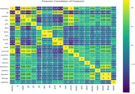
III. CORRELATION BETWEEN FEATURES
Before applying even the most simplest of machine learning algorithms [6], one must work on identifying the various correlations between the features [7] on which these ML algorithms will work on. In our case, we have close to 21 acoustic parameters, understanding their correlations becomes a crucial and time consuming task. We opted to do this task on python and simple Pearson Correlation [8] graph was made (Figire 1.)
Pearson Correlation ranges from -1 to 1
Figure 1. Pearson correlation of features
And it indicates the extent to which two given features are correlated to each other. A value less than 0 indicates that the two features are negatively linearly related. A value of 0 indicates that the two features have no correlation whatsoever. While, a value greater than 0, indicates that the two features are heavily related as the value increases from 0 to 1. Pearson Correlation is calculated via the following formula. Here, X and Y are the features being compared.
One can deduct from the above graph that mean fundamental frequency, minimum and maximum
frequency, and IQR are some of the most important features for out project.
Figure 2
To go a step further, we created scatter plots [10] of the data w.r.t the different features in order to come close to the solutions.
Figure 3. Scatter plot
We can see, some features are accurate in separating the male and female classes while some are unable to do this. Hence, fine tuning is required, and the first step that must be done is to employ logistic regression
[11] analysis to single out the features which work together the best way possible.
IV.IMPLEMENTATION
Baseline Model
To partake whether a given ML algorithm is working better or achieving said results than a non-ML based approach, a baseline model can be used in such cases. The baseline model [12] used in our case responds only to male for the given voice. It does not take into account the acoustic parameters. This baseline model will give us an accuracy of 50% over both training and testing model.
Logistic Regression Analysis
After this, we tried to take a deeper look at the data available to us. We have around 21 acoustic parameters, and to find out parameters with the most significance, a technique known as full logistic regression analysis was applied on the given set of parameters. Our analysis helped us to find out that around 15 out of the 21 acoustic parameters were of statistical significance. This helped us ensure that our model can work with minimal of parameters and not face problems such as overfitting problems.
A logistic regression model from the above analysis gives us an accuracy of around 72% on the training set. On the test set, it gives us an accuracy of around
71%. Clearly, it’s an improvement over the baseline
algorithm and so we can infer that the ML algorithms being applied are working as it should.
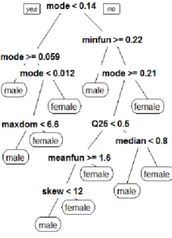
CART
one needs to take into play in order for the model to work upon.
The figure below gives an example of the same.
Figure 4. CART Model
As we can tell from the above CART model, the mode frequency acts as the root node for out CART model. It then moves on to various values of mode and then minimum fundamental frequency, to Q25 and so on until skew. This model gave us an accuracy of around 80% on the training set and 79% on the test set. This has been a bigger boost from the previous logistic regression and the improvement of this CART model could be applied to our Random Forest model, which we plan to use in our project.
Random Forest
Random Forest [14], being similar to the previously applied CART model is of great use to us. We plan to use Random Forest [15] in our project based on its improved accuracy and ease of use through simple modules in R.
After applying it on our given dataset, it freely gives an accuracy of about 100% on the training set and around 88% on the test set. This is again a jump in the improvement of the accuracy of our model.
Support Vector Machine
Next step in our application of algorithm was to try Support Vector Machine [16], also known as SVM. It has to be tuned to best value of gamma and the cost in order for it to work. Hence, this model took the most amount of tuning from its inception to the final version of the SVM which was useful in our project.
To begin with, SVM [17] model was initially made to work on the basic acoustic parameters and simple plot of the obtained SVM model’s error rate was then
plotted. As seen below, shades of blue which are the lightest are the areas where the error rate are the highest and are of no use to us. While, shades of blue which are the darkest indicate the lowest error rates and thus are of good to our model. We will tune the model keeping this in mind.
Figure 5. Performance of SVM (I)
Figure 6. Performance of SVM (II)
We continue this task, after 3-4 passes of fine tuning on the SVM model, we reach on our final model.
Figure 7. Performance of SVM (III)
It gives us an accuracy of around 97% on the training set and gives us an accuracy of 86% on the test set.
We can see this accuracy is only a bit lesser than the Random Forest model we have applied, hence one might assume that the model is not of use. But, since we are planning to use a combination of models known as Stacked/Ensemble, we could use the output of SVM as one of the inputs in the SVM.
XGBoost
XGBoost [18] algorithm could be easily applied on R using a very simple module. Hence we plan to use XGBoost [19] as one of the models in our
Stacked/Ensemble model. It’s an Extreme Gradient
Boosting Algorithm and we plan to use it because of its efficiency, accuracy and feasibility. It has been discussed above in detail.
We’ve been able to achieve 100% accuracy on the training set and around 88% accuracy on the test set. This comes out to be the highest accuracy from all
our models we’ve tested so far.
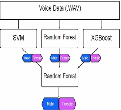
Stacked/Ensemble
We have tried an array of models in the above test cases and found out that the maximum accuracy on the test dataset that could be achieved is around only 88% (through a lot of fine tuning in some models though). To tackle this problem, we use a Stacked/Ensemble [20], i.e. to combine models together in order to boost the accuracy of the newly created stacked model.
In our project we have decided to work with SVM, Random Forest and XGBoost for the Ensemble model. Also, since each different model will give its own classification from the two classes, either male or female, we plan to take the output and feed this again into a Random Forest to again boost the final classification. The final Random Forest will help the ensemble to consider, which of the 3 models is to be given more weight.
Hence, the stacked/ensemble model gives us an accuracy of 89% on the test set.
Figure 8. Stacked Model
V. CONCLUSION
We can conclude that our stacked model which uses the combination of SVM, Random Forest and XGBoost gives us an accuracy of 89% to classify the given voice as male or female. Further improvements applied to the model were simple clocking the analysed frequency between 0 Hz-280 Hz which is the human vocal range [21]. This in turn helped in boosting the accuracy of the models. Further improvements in the model could be the introduction of noise filters to properly clean out the noise from the voice samples. Also, to create a powerful model, introduction of more voice samples in the training of the model could be a tremendous way to improve the accuracy. Currently, we use around 3000 voice samples, but voice samples in the range of say 20000 to 30000 would help us to create a model which is near perfect, given enough diversity is present. Hence, we can say that our model can act as a small stepping stone in a large series of projects in the future.
VI.REFERENCES
[1]. Hassam Ulla Sheikh, University of Manchester, "WHO IS SPEAKING? MALE OR FEMALE" [2]. J. Bishop, & P. Keating, "Perception of pitch
location within a speaker’s range: Fundamental
Frequency, voice quality and speaker sex", in The Journal of the Acoustical Society of America, vol. 132-2, pp.1100-1112, 2012. [3]. R. Vergin, A. Farhat, & D. O’Shaughnessy,
"Robust gender dependent acoustic-phonetic modeling in continuous speech recognition based on a new automatic male/female classification", in Spoken Language, vol. 2, pp.1081-1084, 1996.
[4]. WarbleR Documentation, https://cran.r-project.org/web/packages/warbleR
[5]. Erwan Pépiot, HAL Archives ,"Voice, speech and gender: male-female acoustic differences and cross-language variation in English and French speakers",2013
[6]. Vijayalakshmi A, Midhun Jimmy, Moksha Nair , "A study on Automated Speech Recognition Technique", IJARCET, 2015
[7]. Anjali Pahwa, Gaurav Aggarwal,"Speech Feature Extraction for Gender Recognition", MECS, 2016
[8]. J Benesty, J Chen, Y Huang, I Cohen "Pearson Correlation Coefficient", Springer 2009
[9]. Gelfer, M. P., & Mikos, V. A., "The Relative Contributions of Speaking Fundamental Frequency and Formant Frequencies to Gender
Identification Based on Isolated Vowels",
Elsevier , 2005
[10]. Asuero, A. G., Sayago, A., & González, A. G., "The Correlation Coefficient: An Overview", University of Seville, 2006
[12]. Efron B., "Logistic Regression, Survival Analysis, and the Kaplan-Meier Curve" , JASA , 1988
[13]. De’ath, G., & Fabricius, K. E.,
"CLASSIFICATION AND REGRESSION TREES: A POWERFUL YET SIMPLE TECHNIQUE" , 2000
[14]. LEO BREIMAN, "Random Forests", Machine Learning (Springer), 2001
[15]. Mark R. Segal, "Machine Learning Benchmarks and Random Forest Regression", University Of California , 2003
[16]. CHRISTOPHER J.C. BURGES, "A Tutorial on Support Vector Machines for Pattern Recognition", Springer, 1998
[17]. Gunn S.R., "Support Vector Machines for
Classification and Regression", University Of
Southampton, 1998
[18]. Chen, T., & Guestrin, C., "XGBoost: A Scalable Tree Boosting System" , 2016
[19]. Mitchell R., Frank E., "Accelerating the XGBoost algorithm using GPU computing" , PeerJ , 2017
[20]. Diettrich T.G., "Ensemble Methods in Machine Learning", 2000
[21]. Erokyar H., "Age and Gender Recognition for Speech Applications based on Support Vector Machines", 2014
Cite this Article
Shivangee Kushwah, Shantanu Singh, Kshitij Vats, Mrs Varsha Nemade, "Gender Identification Via Voice Analysis", International Journal of Scientific Research in Computer Science, Engineering and Information Technology (IJSRCSEIT), ISSN : 2456-3307, Volume 5 Issue 2, pp. 746-753, March-April 2019.
Available at doi :