Clustering the results from brainstorm sessions

(1)

Clustering the results

from brainstorm sessions

Master thesis Business Administration

UNIVERSITEIT TWENTE.

Author Jeroen Hek

Student number s1143336

First supervisor Dr. Chintan Amrit

Second supervisor Dr. Mena Badieh Habib Morgan

Specialization Information management

Date 30 July 2014

(2)

(3)

II

Abstract

This research addresses the problem of clustering the results of brainstorm sessions. Going through

all the ideas from the brainstorm session and consolidating them through clustering can be a time

consuming task. In this research we design a computer-aided approach that can help with clustering

of these results. We have limited ourselves to looking at single words and we identify the different

factors that can influence the clustering results. These factors are: (1) word similarity algorithm, (2)

dimensionality, (3) cluster count, (4) clustering algorithm, and (5) the evaluation approach. In total

we tested six word similarity algorithms, two clustering techniques and three evaluation methods, in

order to see which configuration works best for the task. We found evidence that the clustering of

these results is feasible, but the results are influenced by the subjective behaviour of human

(4)

(5)

IV

1. Introduction

This thesis addresses the issue of clustering the results of brainstorming sessions in such a way that

large quantities of ideas can be reduced to a couple of groups. Generating ideas or solutions is the

main purpose of a brainstorm session, however excessively generating ideas can also be a problem

for the technique. While brainstorming, there will be always some overlap of ideas or solutions

within a group, recognizing this overlap and clustering ideas that are similar can be a labour intensive

process, especially when the group size increases. By providing an application that is able to interpret

the results of these sessions and cluster them according to their semantic relationship, this research

will not only be valuable for organizations, but also researchers the application of word sense

disambiguation algorithms on word clusters. It also creates an opportunity for other researchers to

experiment with large scale brainstorm sessions.

1.1. Background

In recent years, organizational brainstorm sessions have been unprecedented popular. The idea is to

yield ideas or solutions from the collective mind of multiple people. Osborn (1953) defines a

brainstorm session as: “To practice a conference technique by which a group attempts to find a solution for a specific problem by amassing all the ideas spontaneously contributed by its members” (p. 151). During a brainstorm session a group or an individual applies a creative technique in order to

find a solution for a specific problem by fabricating a list of ideas. This technique has found its way

into organizations, where it is being used in a collective approach, where not only ideas are being

harvested, but also combined or extended on existing ideas. This generation of new solutions or

ideas has been proven very valuable for organizations.

All brainstorm sessions start with the question about the composition of the panel. Osborn (1953)

proposed the optimum size of this composition is about a dozen, but advocates for an odd number1.

This is to ensure there is the availability of a majority, thus avoiding the danger of creating two equal

sized groups that can obstruct decision-making conferences. Despite the fact that a dozen group

members does not sound that larger, the results of these size groups can still be overwhelming. For

example, the 6-3-5 brainstorming technique where six members write down three ideas every five

minutes. After six rounds the techniques could generate 108 ideas. Osborn (1953) reported that a

session with the American Association of Industrial Editors generated over 400 ideas. This was done

by four panels averaging about 50 members each. Also smaller panels were reported where 28

members produced over 200 ideas.

1_{Although Osborn (1953) advocates for an odd number group size is twelve members still an interesting size.}

(8)

3 The rules of the brainstorming techniques also enhance the creation of new ideas. Below are the

rules according to Osborn (1953) which are briefly discussed.

• Suppress criticism – early judgement against ideas must be withheld;

• Quantity is precondition – the increase of ideas means that the probability of fruitful ideas

increases;

• Combination and improvement – combining ideas can yield something greater than the sum

of the total individual ideas;

• Open minded to unusual ideas – unusual ideas can create new perspectives.

Based on these rules it can be concluded clearly that the technique is all about creating ideas, and

ideally as many as possible. Girotra, Terwiesch and Ulrich (2010) found out that hybrid structures

work better, compared to a group of individuals. In the hybrid structure, individuals first work

individually and then together. The result of this method is that a hybrid structure generated more

ideas and is better for identifying the best ideas.

The main problem with brainstorm sessions is the time consuming task of clustering all the ideas or

solutions that are generated. These sessions are held with relative small groups, as for increasing the

group size will also increase the result count. This increase will further complicate the task of going

through all of the ideas or solution in order to identify major clusters. Thus, to improve this process

there is a need to automatically cluster ideas which will give the brainstorm sessions supervisors a

quick overview about major clusters. These clusters can be used as input for the next brainstorm

session.

The output of brainstorms sessions can consist of single words, multiple words or small sentences

that describe a particular idea. In this research, we have limited ourselves to looking at ideas which

consist of single words. Because of this limitation the choice has been made to look at word

clustering. This is a more fundamental research that can be applied to more problems, than only the

(9)

4

1.2. Research question

The central question for this study is formulated as followed:

“Is it possible to reliably cluster language independent individual words in a given communication context?”

In order to answer this central question, the following questions come to mind:

• Which factors influence the clustering process? • How can the similarity between words be calculated?

Word clustering can be seen as a transformation process. The input will be a list of words and the

output a couple of clusters which contain words that are semantically similar to each other. During

the transformation several steps will be taken, during these steps various factors can influence the

output. Therefore, one of the sub question is to identify which factors influence the transformation

process. Another sub question has to do with word sense disambiguation. Words can be ambiguous

and have multiple senses which only with context get meaning. In this setting there is no context

available, possibly there is a hidden context that the words share with each other. Thus, without

presence of context how can we clusters words without knowing the true word sense.

1.3. Scientific relevance

In recent years the field of word sense disambiguation has been rigorously explored, but has barely

been applied to word clustering. Some scholars have applied word clustering to corpora in order to

cluster words that bear the same specific meaning. The innovative aspect of this research is the

clustering of single words that share a particular context without the presence of context.

Techniques from the field of word sense disambiguation will be applied to the research question and

their individual performance will be measured. This directly leads to the seconds point: how to

evaluate the results of word clustering techniques? Ultimately, human subjects are the only ones

that can assess the quality of these clusters. Thus, this research will elaborate on the transformation

process of word clustering and lay a foundation for this process. In this process several factors will be

identified that can influence the results and will test configurations that produces the best results.

(10)

5

1.4. Social relevance

As brainstorming have become more and more recognized within organization as a method to

construct or synthesize ideas. Although a good session can yield a high return on investment.

Organization will spend a considered portion of time sorting and clustering the results of these

sessions. The organizational relevance of this research is to accelerate this process. The artefact of

this research will proof how a computer can assist this process. Also, because this research looks at

the fundament of word clustering the possibility exists that this can be applied to other problems

where at the heart lies the clustering of words.

1.5. Thesis structure

The theoretical part of the research question will be discussed in chapter two. In this chapter the

numerous techniques how to compute word similarity and word clustering. The chapter start with a

broad discussion of various techniques within the field of natural language processing with respect to

the usage of knowledge bases and afterwards will discuss more in-depth the role of word sense

disambiguation and clustering. In chapter three the execution of the literature review will be

discussed. Followed by the research design used and the implementation of the design to the

research problem. The results of this implementation will be presented in chapter four, and in

chapter five these results shall be discussed. Finally, in chapter six conclusions will be drawn from

(11)

6

2. Theoretical foundation

This chapter describes the foundation for the continuation of this research. It starts out with a broad

discussion about machine learning techniques. Followed by a section about word sense

disambiguation that highlighted how to calculate word similarity and finally clustering. The process of

obtaining all the literature will be discussed first.

At the start of the literature reviews the following scientific search engines were used: Scopus and

ScienceDirect. To obtain a fundamental understanding of the topic a broad search for topic related to

word clustering was performed. The following search terms were used to find articles: (1) word sense

disambiguation, (2) word sense clustering, (3) word clustering, (4) sense clustering, (5) word

similarity and (6) clustering. The subject area filter “computer science” was applied to find specific

articles. While reading the articles bibliography they were investigated to see which sources they use,

articles that were interesting for later usage were collected and added to the literature. The scientific

databases were mentioned before being used to see whom have cited the selected articles. These

studies were examined and, if found useful, added to the literature.

2.1. Machine learning approaches

There are multiple approaches to address the problem of disambiguation, ranging from methods

with a comprehensive body of knowledge or trained data, to methods which do not know the

classification of the data in the training sample. Below are the main learning approaches listed.

• Supervised – makes uses of a training set in which each ambiguous word has been manually

annotated with a semantic label;

• Unsupervised – does not make use of any training data, which could be because it is not

available. The main task of these methods is word discrimination or clustering;

• Semi-supervised – these methods make use of small training set to teach their classifiers; • Knowledge-based – rely primarily on external sources. For example; dictionaries, thesauri,

ontologies, collocation, etc. which are used to infer the word sense of the target word from

the context it belongs to.

2.1.1. Supervised

Supervised learning is a machine learning task in which a disambiguated corpus is used to train the

algorithm (Manning & Schütze, 1999). The training data typically contains a set of examples. In these

examples each occurrence of the ambiguous word is manually annotated with a semantic label. The

classifier analyses the training data to produce an inferring function, which can be used to correctly

(12)

7 better results compared to unsupervised methods. However, it costs a substantial amount of manual

labour to sense-tag a corpus for training, which can form a bottleneck for the learning method. In the

next subsection a couple of supervised methods will be reviewed.

Bayesian classification

A Bayes classifier looks at the words around an ambiguous word in a large context window (Manning

& Schütze, 1999). The idea is that each piece of content can contribute potential useful informative

to determine the sense of the ambiguous word. The Bayes classifier is a statistical classifier which

applies the Bayes decision rule that minimizes the probability of error when choosing a class

(Manning & Schütze, 1999). This is done by choosing the sense with the highest conditional

probability, thus minimizing the error rate.

Naïve Bayes

The Naïve Bayes classifier is an instance of a Bayes classifier (Manning & Schütze, 1999), which uses a

simple probabilistic classifier. The Naïve Bayes classifier is a widely used supervised machine learning

method based on the Bayes’ theorem. It is widely used due to its efficiency and ability to combine

large numbers of features. The method is called Naïve Bayes because of the “naïve” assumption of

independence between features. This assumption has two consequences: (1) the first is that

structure of the words within the context is ignored, and (2) the presence of one word in the context

is independent of another. This assumption that all features contribute independently is clearly not

true (Manning and Schütze, 1999). Terms are conditionally dependent on each other. Despite its

incorrect assumption the model can be quite efficient. Navigli (2009) describes the inner workings of

the model as follows: “It relies on the calculation of the conditional probability of each sense Si of a

word w given the features fj in the context”. The word sense which maximizes is chosen as the most

as the most appropriate in this context.

= _∈

|

Information theory

The Bayes classifier looks at the context windows around the ambiguous word to determine the

correct word sense, while having an unrealistic independence assumption. The information theory

algorithm takes a different approach. Manning and Schütze (1999) describe this approach as: “It tries

to find a single contextual feature that reliably indicates which sense of the ambiguous word is being

(13)

8

Decision list

According to Navigli (2009) a decision list is: “an ordered set of rules for categorizing test instances for assigning the appropriate sense to a target word”. This list exists of rules which behave like an “if-then-else” statement, where each of the rules is weighted. A training corpus is used to extract a set

of features. This results in rules of the kind (feature-value, sense, score) and will be ordered based on

their decreasing score. The method is based on ‘One sense per collocation property’, which status that word surrounding the ambiguous word provide strong clues about the correct word sense. As

like in the Naïve Bayes method the word sense with the highest score will be assigned to the

ambiguous word.

= ∈ !!"# $%

Decision tree

A decision tree is a predictive model used to represent classification rules with a tree structure that

recursively partitions the training data set. Each internal node of a decision tree represents a test on

a feature value, and each branch represents an outcome of the test. A prediction is made when a

terminal node (i.e., a leaf) is reached.

A decision tree, like the decision list, behaves like an “if-then-else” statement. The only difference is

the hierarchical positioning of features. Each internal node represents test on a feature, each branch

represents outcome of test and each leaf node (terminal node) represents class label. A word sense

will be assigned when the leaf node has been reached. Manning and Schütze (1999) stated that the

C4.5 algorithm is a popular one for decision trees, although they are outperformed by other

supervised approaches.

Support Vector Machine

Support Vector Machines (SVM) constructs a linear hyperplane from the given training set and

categorizes the examples to one of two categories, which makes it a binary linear classifier. The SVM

model represents a point in space where the gap between the separated categories is as wide as

possible. The data points lying closest to the hyperplane are considered to be the support vectors.

The model is comprised of two elements: (1) a weight vector, and (2) the bias. If the training set is

non-separable slack variables can be used to allow the model to separate the space, thus create a

linear hyperplane.

2.1.2. Unsupervised

Supervised approaches make of a training set of examples to train their classifiers. However, there

(14)

9 available lexical resources are lacking. The challenge for unsupervised methods is to overcome the

lack of resources. According to Manning and Schütze (1999) complete unsupervised disambiguation

is impossible. Although, sense discrimination can be performed completely unsupervised. This

approach is called ‘clustering’. Manning and Schütze (1999) describe this discrimination task as follows: “one can cluster the contexts of an ambiguous word into a number of groups and discriminate between these groups without labeling them”. Navigli (2009) adds that these discrimination tasks may not create equivalent cluster compared to traditional sense clusters found

in a dictionary. This makes it difficult to evaluate these methods. A solution could be to ask humans

to assess the nature of the relationship between members of each cluster. In their purest form

unsupervised methods do not make use of any machine-readable resources like dictionaries,

thesauri, ontologies, etc.

2.1.3. Semi-supervised

Supervised and unsupervised approaches above are on the extreme side of the line. Where

supervised approaches have a training set were ambiguous words are manually annotated with their

semantic label and, unsupervised approach does not have any training data. Between these two

approaches there are also methods which use a small annotated training set to train the classifier. In

this subsection the popular method bootstrapping will be discussed.

Bootstrapping

Bootstrapping is a method to build a classifier with little training data and iteratively improve the

classifier’s performance. One of the problems to overcome is the lack of annotated and scarcity of

data (Navigli, 2009). Yarowsky (1995) describes the method as: “one begins with a small set of seed examples representative of two senses of a word, one can incrementally augment these seed examples with additional examples of each sense, using a combination of the one-sense per- collocation and one-sense-per-discourse tendencies”.

The annotated data of the classifier grows through including the most confident classification found

in the untagged corpus. Resulting in a shrinking training set, until a certain threshold (e.g. iterations)

is reached. Yarowsky (1995) advises several strategies to which could form the initial seed:

1. Use words in dictionary definitions – entries from a dictionary already appear in the reliable

relationships with the target word;

2. Use a single defining collocate for each class – only use context with have a single definition

of a the target word;

3. Label salient corpus collocates – words that co-occur with the target word tend to be

(15)

10 The method avoids the need for costly manually annotated data by exploiting two properties of the

human language:

• One sense per collocation – Words nearby the target word strongly and consistently

contribute to the sense of the word, based on their relative distance, order, and syntactic;

• One sense per discourse– word sense of a target word is consistent within any given

discourse or document;

The advantage of this method is that the addition of untagged data to the label data set (Navigli,

2009). Yarowsky (1995) posit the method is more sensitive, compared to typical statistical

sense-disambiguation algorithms, to a wider range of language detail. According to Navigli (2009) one of

the disadvantages is the lack for select optimal parameters (e.g. pool size, number of iterations, and

number of most confident examples).

2.1.4. Knowledge-based

Knowledge-based or dictionary-based learning exploits knowledge resources when there is no

information about the sense of the target word. Resources such as dictionaries, thesauri, ontologies,

collocations, etc. are used to infer from context the senses of words (Navigli, 2009). Compared to the

supervised approach this approach performance is lower, but has the advantage to cover a wider

range due to the usage of knowledge resources. However, recently some researchers reported that

knowledge-based techniques match the performance of supervised techniques (Navigli, 2009). In the

following subsections several knowledge-based approaches will be discussed.

Selectional Preferences

Selectional preferences exploit the number of meanings that a target word could possess in context.

Restrictions are imposed on the semantic classes of words co-occurring with the target words, thus

constraining the denotation of the direct object. For example, the word ‘ride’ expects an inanimate object as direct object. The direct object must also be denoted as for example ‘vehicle’.

Structural Approaches

With the arrival of lexicons, like WordNet (Miller, Beckwith, Fellbaum, Gross, & Miller, 1990), several

structural approaches have been developed. These approaches exploit the structure of the concept

network within the lexicon and analyze the structure interrelationship between senses based on

features. Recently, the structural approach using WordNet has found the attention of many scholars

(Voorhees, 1993; Agirre & Rigua, 1996; Altintas, Karsligil & Coskun, 2005; Tsatsaronis, Vazirgiannis &

(16)

11 is that WordNet can be used as a machine readable dictionary that beside definitions can also

contain a hierarchical structure. In the next chapter the benefits of these functions will be discussed.

Thesaurus-based disambiguation

The method thesaurus-based disambiguation exploits the subject categories supplied by a dictionary

or the semantic categorization from a thesaurus. Navigli (2009) describes the method as follow: “The basic inference in thesaurus-based disambiguation is that the semantic categories of the words in a context determine the semantic category of the context as a whole, and that this category in turn determines which word senses are used”.

2.1.5. Summary

The literature is not really clear on when to use a supervised, semi-supervised or unsupervised

approach. If there is knowledge available (i.e., manually labelled test data) then they argue to use the

supervised approach. Otherwise you should choose for one of the other approaches. Also, the other

parameters come in to play when choosing an approach, namely: time and the kind of problem. As

stated by Manning and Schütze (1999), if the kind of problem is the clustering of data, a supervised

approach is ideal for solving the problem.

Looking at the performance of the different approaches, it is noticeable that the supervised approach

triumphs in machine learning. The performance is almost unmatched, nevertheless this performance

comes with a huge cost and which is the obtainment of manually labelled training data. This is a time

consuming and expensive task. Recently researchers reported that semi-supervised or knowledge

based techniques show promising result for several reasons (Navigli, 2009). First, the more

structured knowledge is available, the better the performance of these techniques will be. Second,

knowledge-based resources used are increasingly enriched (i.e. the evolution of WordNet). Third, the

potential of domain ontologies can be exploited by knowledge-rich techniques.

For this research the used method of machine learning approach, depends on the analysis of the

word sense disambiguation techniques. During the selection mentioned earlier, parameters will be

taken into consideration. In the following section several word disambiguation techniques will be

discussed and compared to another. Depending on the results a method will be chosenfor the

(17)

12

2.2. Word sense disambiguation

Disambiguation is an intermediate task, because it is necessary to accomplish certain tasks. First a

short description of Word Sense Disambiguation (WSD) will be elaborated on, giving a definition and

the application of the task. Next there will be an overview of existing literature regarding WSD will be

discussed. Finally, several algorithms will be selected and compared to each other.

Ambiguity is common in the human language, so determining the meaning of a particular word

depends on the context the word occurs in. As an example of ambiguity, take the word ‘match’, WordNet comes up with multiple meaning to the word:

• Lighter consisting of a thin piece of wood or cardboard tipped with combustible chemical;

ignites with friction;

• A formal contest in which two or more persons or teams compete; • A person who is of equal standing with another in a group;

• Something that resembles or harmonizes with.

For word sense disambiguation it is the task to identify which sense (i.e. meaning) of a word is used

in a sentence, when the word is ambiguous. Manning & Schütze (1999) describes the task as: “The task of disambiguation is to determine which of the senses of an ambiguous word is invoked in a particular use of the word”. According to Navigli (2009) the task implies: “Word sense disambiguation is the ability to computationally determine which sense of a word is activated by its use in a particular context”. Context surrounding the word is used to determine the sense of a particular ambiguous word.

WSD has a broad application. Within machine translation words can have different translations in

different sentences. For example a English-Dutch translator could translate the English noun ‘full’

translated to ‘volledig’(complete) or ‘verzadigd’(saturated). It could also benefit information retrieval system to interpret the given query. For example, the query ‘bar’ should the system return information about nearby retail establishments where they serve alcoholic beverages or describe

something about the atmospheric pressure. Disambiguation is beneficial and most of the time even

(18)

13

2.2.1. Approaches

Not only can WSD approaches are categorized as supervised or unsupervised. The approaches belong

to one of the two main approaches that have previously been identified: (1) text-based approach and

(2) structure-based approach (Altintas, Karsligil & Coskun, 2005, Sebti et al. 2008).

• The text-based approach uses a large corpus or word definitions to collect statistical data in

order to calculate an estimated score of semantic similarity;

• The structure-based approach relations and the hierarchy of thesaurus of lexical database,

which are generally hard-crafted such as the lexical database WordNet of the Roget’s

Thesaurus.

In the following subsections several text- and structure-based approaches will be discussed.

2.2.1.1. Edge-based approach

According to Jiang and Conrath (1997) the edge-based approach “is a more natural and direct way of evaluating semantic similarity in a taxonomy”. The approach calculates the distance between words (nodes) in order to measure the similarity between words. Hierarchical taxonomy, like WordNet, can

be used to calculate similarity distance. Obviously, the smaller the distance between two words the

more similar they are to each other. Methods penalize hierarchical depth as described below. The

higher the shared concept of two words is positioned in the hierarchical tree the less the words will

be similar.

Voorhees (1993) used the ‘IS-A’ function of WordNet to determine the true sense of words in

information retrieval systems. The ‘IS-A’ function returns the hyponym of a sense (i.e. car IS-A

vehicle). With the use of only the ‘IS-A’ function, it could be used to determine word sense, although

the degradation of performance is due to the small context window in the query (Voorhees, 1993). It

is complicated to determine the correct word sense when there is little or no context to make use of.

The usage of WordNet increased due to its semantic relations with the database. The latest versions

of WordNet offers relations like: hypernymy/hyponymy, meronymy/holonymy,

synonymy/antonymy, entailment/causality, troponymy, domain/ domain terms, derivationally

related forms, coordinate terms, attributes, and stem adjectives. Many scholars saw the value of

these relationships. As like Voorhees (1993), Wu and Palmer (1994) used the relationship structure

from WordNet to calculate sementic similarity. Semantic similarity of two words is calculated based

on their path length between the two words. Wu and Palmer (1994) used the follow formula to

(19)

14

&%'&, &) =_, 2 × , + ,)+ 2 × ,

-• &_- is the least common hyponym of & and &₎.

• , is the length of the path (number of nodes) from & to &_-. • ,₎ is the length of the path &₎ to &_-.

• , is the path length from & to root.

Wu and Palmer (1994) reported accuracy between 57.8% and 99.45%. The approach applied by Wu

and Palmer (1994) is called edge-based. The main premise of this approach is; the shorter the path

between two nodes the more similar they are.

This concept of path length between words was also used by Agirre and Rigua (1996) whom

introduces the conceptual distance approach. According to Agirre and Rigua (1996) this approach is

comparable with the approach of Resnik (1995). It calculates semantic similarity based concepts in

the hierarchical of WordNet. The approach focus on nouns and looks at; path length between nodes,

depth of the nodes and node that subsumes the nodes and the density of the hierarchy.

&/$, =∑ ℎ23

4.64

7 8

9$9:;

Where $ is the concept that is at the top of a sub-hierarchy, and ℎ23 is the mean number of

hyponyms per node. Agirre and Rigua (1996) reported accuracy between 53.9% and 71.2%.

Another approach that uses the hierarchy of WordNet is that of Altintas, Karsligil & Coskun (2005).

They propose an approach that is comparable to the approach of Wu and Palmer (1994). According

to Altintas, Karsligil & Coskun (2005) “concreteness and abstractness are attributes of concepts which can help us improve our estimations when calculating similarity of concepts”. Path length between words alone does not provide information about their similarity. By including the depth of the word

and the depth of the word that subsumes the two words, they are able to differentiate between

words to result in a better similarity score. The similarity function is defined as followed:

', ) =_{1 + =$:% + 3$$:%}1

Where the =$:% is:

(20)

15 The ℎ%:= is the shortest path between the two given words and the >%%2/3:ℎ is the

deepest words in the taxonomy. The other parameter in the similarity function is the 3$$:%.

This is the difference between the specificities of the two words. This is calculated as followed:

3$$:% = ?3$ − 3$)?

Where;

3$ =_&AB:/3:ℎ/3:ℎ

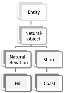
The 93:ℎ is the depth of the word in question (i.e. the depth of the word ‘Entity’ is zero). The

&AB:/3:ℎ is depth to the node which both words share. Altintas, Karsligil & Coskun (2005) report an accuracy that is better compared to that of Wu and Palmer (1994).

2.2.1.2. Node-based approach

The node-based approach determines word similarity based upon the information-content approach

(Jiang & Conrath, 1997). The term Information Content (IC) was posit by Resnik (1995) and calculates

the word probability in a given corpus. The node-based approach takes the least common ancestor

and calculates its IC value. The concept of information-content will be discussed in depth and several

node-based approach will be discussed below.

Resnik (1995) introduced the concept Information Concent (IC). The IC value is the probability that a

concept occurs in a given corpus. This value is calculated by the negative log likelihood formula:

C&$ = −A%3$

The idea behind quantifying information concept is based on the appearance of words in a corpus. As

the probability of appearance increases the information the words carriers decreases, making the

word a more abstract concept. Therefore, infrequent words convey more information compared to

frequent words. Semantic similarity is calculated as follows:

'$, $) = max_{; ∈ ;}

G,;6 C&$

The more information two words have in common, the more two words are similar to each other.

Jiang and Conrath (1997) combined the information content approach of Resnik (1995) with the

edge-based approach. Next to the log probability of the concepts, the method also uses the least

(21)

16

', ) =_−A%3 1

− A%3) + 2 × log3=&K + 1

Like the above method , Lin (1998) combined the information content approach of Resnik (1995)

with the edge-based approach as well.

', ) =_{log 3}2 × A%3=&K + log 3)

Both methods state that if two concepts are identical the outcome will be one, when it is zero the

two concepts have no common features. Jiang and Conrath (1997) and Lin (1998) compare their work

to that of Miller and Charles (1991), which resulted in a .828 and .834 correlation respectively.

Based upon the Information Content of Resnik (1995) Sebti and Barfroush (2008) propose an

approach of calculating semantic similarity using the hierarchical structure of WordNet. According to

Sebti and Barfroush (2008) they improved the approach of IC with adding the edge counting-based

tuning function and reported an accuracy that is higher compared to that of Wu and Palmer (1994)

and Resnik (1995).

2.2.1.3. Corpus-based approach

Corpus-based disambiguation approaches are usually semi-supervised, because they use

pre-annotated data that has been made by people to serve as training data. Other corpus-based

approaches use large corpora to calculate word distances . These distances, or cosine distances,

between words allow the algorithm to say something about word similarity by watching how often

they share the same context.

Tsatsaronis, Vazirgiannis and Androutsopoulo (2007) combined the spreading activation network,

and applied a weighting scheme to their approach. The weighting was applied to the edges of the

network and used the term frequency and inverse document frequency also known as TF-IDF to

calculate the weight for the edges. The TF-IDF approach is a statistical approach which is often used

in information retrieval and text mining. It looks at the term frequency, which can increase

proportionally depending on the document, although the inverse document frequency helps to

control for the occurrence of words. Words that occur less are more valuable according to the

approach compared to words that occur often. Compared to the approach of Véronis & Ide (1990)

the approach of Tsatsaronis, Vazirgiannis and Androutsopoulo (2007) does score a better accuracy,

namely between 34.3% and 38.7%. Although the results of the approach look promising the

computational complexity is one of the disadvantages of the approach. According to Tsatsaronis,

(22)

17 higher compared to other techniques. This complexitiy is a result of the network the technique

builds, in which it includes almost the entire dictionary. Another neural network approach is

suggested by Mikolov, Sutskeven, Chen, Corrado and Dean (2013). They have introduced a

continuous Skip-gram model that efficiently learns high-quality distributed vectors that represent a

large number of syntactic and semantic relationships. The model predicts words within a certain

window surrounding a target word. Distant words are less related to the target word and were given

less weight, compared to words that are closer to the target word. Mikolov et al. (2013) found that

high dimensional word vectors can be used to answer subtle semantic relationships between words.

This will tell if words are similar to each other, but also answer questions like: A is like B as C is to D

where D will be given by the system (e.g., France is to Paris as Germany is to X, the system will return

‘Berlin’ as answer).

Cowie, Guthrie and Guthrie (1992) proposed an approach called Simulated Annealing which

determines the word sense of a target word using the complete sentences in which the target word

operates. The rational of using the context of the target word is that senses that belong together

have more words in common with their definitions compared to senses that do not belong together.

The approach is comparable to that of Lesk (1986) only here the context of the surrounding word is

used to measure overlap in contrast of the definition of other words. According to Cowie, Guthrie

and Guthrie (1992) the results are comparable to that of other co-occurrence approaches.

Several scholar also cluster word using corpora (Purandare & Pedersen, 2004; Deepak, Roa &

Deepak, 2006; Sugiyama & Okumura, 2009; Zhu & Lin, 2009; Broda & Mazur, 2010; Martín-Walton &

Berlanga-Llavori, 2012). The input of these algorithms is a corpus and the output are word clusters

contain words that share a similar context with each other. This approach is highly dependent on the

context surrounding the words, otherwise it would not know how words are related or differentiate

word senses.

2.2.1.4. Other approaches

Dictionary and thesaurus based

Lesk (1986) proposed an approach in which the definition of a word was used to determine the true

word sense of a word. He used the Oxford Advanced Learner’s Dictionary of Current English to gather

the word sense of several words and calculated the overlap between definitions. He took a ten word

window around the target word and calculated the overlap. The word sense with the highest overlap

(i.e. words that appear in both definitions) is presumed to be the correct one. For example, ‘bank’ in

(23)

18 ‘a slope’ or ‘body of water’ the word belongs to steep natural incline. The overlap between the senses and the dictionary definitions is calculated by counting words that occur in both sentences.

$%P!Q = , ) =|A% ∩ A%)|

Where A% represents the bag of words in the context surrounding the target word and the dictionary definition. The algorithm assumes the correct sense to be that which has the highest

overlap. The accuracy of the algorithm scores between 50% and 70% when applied to a sample of

ambiguous words. A disadvantage of the overlap function is its sensitivity to the exact wording of

definitions.

The neural network approach by (Véronis & Ide, 1990) combines the use of machine readable

dictionaries, spreading and activation models. The latter places words (nodes) into a network that

can be described as a neural network. These nodes are connected to each other by ‘activatory’ links

that activate concepts which are related to the words. In addition ‘inhibitory’ links usually

interconnect competing senses of a given word. The system builds a network based upon words

which after a while grows to almost the size of the dictionary, because of all the relations word

senses contain. The second step is to activate the words which need to be disambiguated. Each node

activates their neighboring words until the entire network has been activated. Inhibitory links sends

inhibition to one another. This strategy activates related words and deactivates unrelated or weakly

related nodes. Véronis & Ide (1990) found that their approach works better compared to that of Lesk

(1986). The approach of Lesk fails to disambiguate the right sense with the words: pen and page.

According to Véronis & Ide (1990) the approach is more robust, because it does not rely on the

occurrence of words in word sense definitions.

Because of the sensitivity of the overlap function researchers looked for other possibilities that could

be used to compute semantic similarity. Yarowsky (1992) used the Roget’s thesaurus in which he

identified and weighted words that could indicate the sense of a word in context. The statistical

approach used a window of fifty words surrounding the target word. The correct sense was the one

which has the highest sum. Beside the overlap and statistical similarity researchers also looked at the

structural similarity between word senses. Yarowsky (1992) uses the Bayes’ rule to calculate the

probability of the senses and determines the right sense where the sum is the greatest. The formula

used is displayed below.

KSTUKV

(24)

19 Kolte and Bhirud (2009) continued to build on the work of Lesk (1986). They have stated that the

overlap function suffers from the definition size in WordNet, which is too small. In order to improve

the approach of Lesk (1986) additional definitions are collected from Hypernymy and Hyponymy.

These definitions are added to the bag of words. In addition to the hypernymy and hyponymy

functions Kolte and Bhirud (2009) also research the impact of other WordNet function, namely:

Meronymy / Holonymy, ability link, capability link and function link, although they do not report their

findings of these functions. Their disambiguation approach has an accuracy of 63.92%.

Semi-supervised and supervised approaches

There are also approaches with could be categorized as semi-structured due to their usage of

sources. Sources like: NY Times corpus, Brown corpus, Wikipedia or other dictionaries. These

approaches train their classifier on these data sources and then present the classifier with a words or

sentences to disambiguate. The approach from Yarowsky (1995) is a prime example for a

semi-supervised approach. The approach uses a large corpus to train their classifier. From the corpus the

classifier learn the context from words by looking at the window around the words. These windows

are stored and used to compare against new context windows from which the classifier can

determine the true sense of the target word. According to Yarowsky (1995) this semi-supervised

approach scored surprisingly well, reporting accuracy scores around 72% and displays scores that are

similar to supervised approaches.

Supervised disambiguation techniques make use of manually labelled test data. As stated before, this

need for manually labelled test data is one on the disadvantages, as is it hard to obtain these

resources, although some scholars reported very high scores using this approach. Like Ng and Lee

(1996), they have trained their classifier with a corpus in which the senses were pre-tagged with the

correct senses. When given unseen sentences the classifier matches it against the training data and

uses the best match to determine the sense of the target word. The difference between pre-tagged

and untagged data is directly visible in the results the classifiers produce. The supervised classifier

score 89% accuracy, which is much higher compared to that of Yarowsky (1995). However, as

mentioned before, this difference in performance comes at a price and that price is the time

consuming task of pre-tagging training data. Some scholars also tried to combine supervised and

unsupervised techniques. Agirre, Rigau, Padró and Atserias (2000) used lexical knowledge sources

and combined these with supervised training corpora to enhance their technique. The unsupervised

technique alone had an accuracy between 41.6% and 43.6%, when this was combined with the

(25)

20 Another example is the approach of Schütze (1997) where news data from multiple sources was used

to train their classifier. Similar to Yarowsky (1995) approach it is automatic and can be supplied

untagged news data to train the classifier. The approach creates word vectors from words that are

close neighbors within the training corpus and neighbors that co-occur within the large window

surrounding the target words. Similarity is then calculated by measuring the cosine between these

two vectors. This cosine measure can be compared to the normalized correlation coefficient.

Wikipedia

Another knowledge source that has recently caught the attention of researchers is Wikipedia.

Wikipedia is a multilingual free internet encyclopedia that is maintained by volunteers. Anyone can

access the site and edit almost every article. At the moment Wikipedia contains 30 million articles in

287 languages and the English section of Wikipedia has over 4.4 million articles. An article typically

defines and describes an entity or event and has hyperlinks to other entities or events. Mihalcea

(2007) uses the hyperlinks within Wikipedia. For example, the word bar could mean law or music and

are stored in the articles as piped links (i.e., [[bar (law)|bar]] or [[bar (music)|bar]]). Mihalcea (2007)

states that these piped links can be regarded as sense annotations for the corresponding concepts

and the content of the articles as the context of the concept. Wikipedia also has disambiguation

articles which consist of links to different articles that define different meanings of a concept.

Although, these pages were not used due to their incompleteness and inconsistency how

disambiguated pages are been used2. The first step of the disambiguation process is to collect the

piped links of the target word and the related article. In the final step the window around the target

word is used to calculate co-occurrence against the Wikipedia articles to determine the correct word

sense. Mihalcea (2007) reported accuracy between 79% and 85%.

2.2.2 Summary

As stated by Ide and Véronis (1998), word sense disambiguation is an intermediate task, which

means that it is a necessary task to perform in order to accomplish another task. This is also the case

with the artifact. First, the correct sense of a word needs to be determined, otherwise clustering of

these words would become difficult. It has to be noted that disambiguation is not the primary goal is

of this research and other techniques can have a different effect on the cluster results.

The main problem in this research with regard to disambiguation of single words is the lacking

context which can be used to determine the sense of a word. Most techniques discussed in this

2

(26)

21 thesis make use of a window surrounding a target word. The reason is that the word sense can be

identified by the company the word is surrounded by. This lacking context will definitely have an

effect on the accuracy of the disambiguation process. However, the question asked during a

brainstorm session will give certain direction to a particular context , this context will be hidden in

the relation the words have with each other. Therefore it can be stated that there will be a latent

context within the results of a brainstorm session.

Several techniques have been discussed in the section above. Edge-, node- and corpus-bases

techniques are the most commen used in the field of word sense disambiguation. All approaches use

different resources to train their classifier and achieve different results. Resulting in no clear answer

to the answer of which resource provides the best result. Overall, it can be stated that supervised

techniques perform better compared to unsupervised techniques. The knowledge-based techniques

score relative high and, as stated before, almost match the results of supervised techniques.

The spreading activation network models show real potential despite their complexity. Parameters

such as tuning, thresholds and decay make the techniques difficult to use. Another disadvantage is

the high processing complexity. Compared to other techniques the network model uses more

resource. For these reasons the spreading activation network techniques will not be used in the

artifact.

Semantic similarity techniques seem interesting due to their simplicity and reported accuracy.

Several WSD algorithms result in almost similar scores, but none of these have ever been applied in

the task of word clustering. Therefore, several techniques will be selected and compared to each

other in order to measure performance during the clustering task. The edge- and node-based

approaches provide very promising results and of these approaches the following will tested:

• Edge based

o Wu and Palmet (1994)

o Altintas, Karsligil & Coskun (2005)

• Node based

o Resnik (1995)

o Jiang and Conrath (1997)

o Lin (1998)

From the corpos-based approach the technique of Mikolov et al. (2013) will be used. The authors did

not perform any WSD experiments, but it shows promising results for word similarity. Especially with

(27)

22 vectors in order to determine what the cosine distances are relative to other words. These vectors

can also be used to measure word similarity. The advantage of this approach is that it is not tied to a

vocabulary that is pre-determined by other people (i.e. WordNet and other dictionaries). This allows

the application domain to read specific texts to expand its vocabulary.

When looking at the evaluation of the different techniques the conclusion can be made that none of

them are really applicable to this study. Most of the edge- and node-based techniques use the

research from Miller and Charles (1991). They asked 38 students from the University of New York to

rate 30 noun pairs on their similarity. They were instructed to give a rating from zero to four, where

zero represents no similarity and four perfect similarity or synonymy. This resulted in a list that

represents the semantic similarity between the noun pairs. The edge- and node-based algorithms use

this research to calculate correlation between their similarity rating and that from Miller and Charles

(1991). The word-sense induction techniques compare their results to pre-annotated data, like

SENSEVAL3 (renamed to SEMEVAL) or other knowledge bases. Others used humans to evaluate the

findings of their research, because when it comes to language humans are to only subjects to set the

golden standard. Because of the lack of an established evaluation metric an fitting evaluation

procedure needs to be designed in order to capture and compare performance for each of the

algorithms. Advisable is to make use of human informants, because of their skill to determine if

words belong to the correct cluster (Gale, Church & Yarowsky, 1992).

2.3. Clustering

In this chapter we will investigate several cluster techniques in order to answer the sub-research

question: “In what way can cluster techniques be applied?”. In the following subsection several techniques are identified and reviewed to see under which conditions they work, also their

advantages and disadvantages of each method will be discussed.

For example, if we cluster English nouns according to their syntactic and semantic environment the

days of the week will end up in the same cluster, because they share the environment

‘day-of-the-week’. Another method to measure word similarity is by looking at the distribution of the

neighbouring words, for the two target words and calculates the degree of overlap. Manning and

Schütze (1999) advice to spend some time getting familiar with the data at hand, and state it is a

mistake to skip this part. When there is no pictorial visualization for linguistic object, clustering could

be an important technique in exploratory data analysis (EDA). Clustering techniques can be

differentiated into two categories, namely: (1) soft clustering, and (2) hard clustering. Hard clustering

techniques allocate each individual object to only one cluster, where soft clustering allows objects to

3

(28)

23 be a member of multiple clusters. Mostly clustering techniques use hard clustering, but according to

Manning & Schütze (1999) most soft clustering techniques allocate object to only one cluster. Hard

clustering techniques have to deal with uncertainty if the assigned cluster is truly the correct one for

each object. There always exists the possibility individual object belong to more than one cluster. A

true multiple assignment technique is called ‘disjunctive clustering’, in object can be assigned to several clusters and also truly belong in those clusters. Manning & Schütze (1999) identified two

main structural categories where clustering techniques belong to, namely: (1) hierarchical clustering,

and (2) flat clustering techniques. With flat clustering objects are distributed over several clusters,

although the relationship between the clusters could not be determined. In hierarchical clustering

each node stands for a subclass of their mothers’ node, where the leaves of the tree represent

elementary clusters. In the next subsections we will discuss several methods belonging to the two

main structural categories. Evaluation of clustering results will be discussed in 3.3.1.

2.3.1. Hierarchical Clustering

The bottom-up algorithm, also called agglomerative clustering, start with putting each individual

object in a separate cluster. Each iteration clusters two most similar clusters which are determined

and combined into a new cluster. This process continues until one large cluster has been created

containing all objects. Compared to the bottom-up algorithm, the top-down algorithm, also called

divisive clustering, start with placing all the individual object in one large cluster. Each iteration the

algorithm determines which objects least similar and splits these objects into new clusters. This

continues until each individual object has been separated from their parent cluster. At the end of

these algorithms the root of the tree exists of one large cluster which holds all objects, the branches

are the clusters, and the leaves exists out of the individual objects.

The algorithms discussed above are part of collection methodologies which describe a particular way

of hierarchical clustering. The full list of methods is:

• Single-link – most similar objects are clustered together, like the agglomerative clustering; • Complete link – least similar object are clustered, like the divisive clustering;

• Group-average – by measuring mean distance between objects and clusters.

In the following subsections these methodologies will be discussed.

Single-link clustering

The single-link cluster follows the same clustering technique as the agglomerative clustering. Objects

which are most similar are cluster together until a cluster is created which contains all of the

(29)

24 Schütze, 1999). The MST connects objects with span equal to or less than every other spanning tree.

Thus, the smallest span between two objects equals to the largest similarity. The advantage of the

single-link clustering is its complexity, which is L), because every object has to be examined at least once.

Complete link clustering

Where single-link cluster is looking at the maximum similarity between two objects, the complete

link cluster uses the negative of this function, thus the minimum similarity. The technique could use

the MST, although instead looking for objects which tree spanning is the smallest, complete-link

clustering removes objects with the largest span from the cluster. The disadvantage of this technique

is its time complexity L-, since there are merging steps. Each step of the algorithm requires

L)_{to find the largest distance between two object.}

Group-average clustering

A compromise between the single-link and complete-link clusters is called group-average clustering.

This technique does not look at data points which are closest and/or furthest separated from each

other, but the clusters are based on the average distance between objects within two clusters and

merging those which are closest related. The time complexity is the same as that of the single-link

technique, thus L). This could be L- when the average similarity is calculated each time two group were merged.

2.3.2. Non-Hierarchical Clustering

Non-hierarchical cluster methods create cluster by distributing objects into clusters from a data set

which (generally) have a non-overlapping group and no hierarchical relationship between them. An

advantage of non-hierarchical methods is the lower demand on computational resources. Compared

to hierarchical methods the time-complexity will typically be L or L). Although, most methods employ multiple passes to reallocate object and refine the result, which will put pressure on

the resources. This also raises the question: If multiple passes are needed, when does the algorithm

stop working? According to Manning & Schütze (1999) there is one possibility which can be used to

determine the stopping criteria is the validity of the cluster’s quality. The group-average similarity

method can be used to measure this quality. Beside of the validity of quality’s problem, there is also

the question of the right amount of clusters.

In the following subsections two popular algorithms will be discussed, namely: (1) K-Means, and (2)

(30)

25

K-Means

Manning and Schütze (1999) define the K-means algorithm as: “a hard clustering algorithm that defines clusters by the center of mass of their members”. The algorithm needs an initial cluster count

M which needs to be defined by the user. From the data set M data points are used by the algorithm as initial means. Next an iteration process start where each of the iteration objects are assigned to

their closed cluster. After every object has been assigned, a new cluster mean, or centroid, will be

calculated. A centroid is the average of all members belonging to a specific cluster, also known as a

hypothetical cluster object, although these averages are sensitive for outliers. Manning and Schütze

(1999) stated that the use of medoids are less sensitive for outliers, for this in one of the objects

within cluster. Also, instead of using the sum of the squared Euclidean distance, K-means algorithms

using medoids minimizes the sum of pairwise dissimilarities. The time complexity is L because each iteration distance from each object to the cluster center is calculated and minimal distance

determines the object membership of a cluster. A problem arises when objects have equal distance

to multiple clusters. One solution is to randomly assign the object to one of the clusters, although

this has the disadvantage that the algorithm may not converge (Manning & Schütze, 1999).

Expectation-Maximization (EM)

Compared to the K-means algorithm is the EM algorithm a soft clustering method. The task of the

algorithm is to find the maximum-likelihood estimate of the hidden parameters of an underlying

distribution (Manning & Schütze, 1999). For each object the probability that it belongs to a cluster

and the one with highest probability will be the cluster that object is assigned to, but the object will

still have a non-zero membership to all the other clusters. The algorithms follow an iterative process

where it calculates the expected membership probability under given parameters and in the second

step tries to maximizes this quantity. Advantages of this technique is the possibility of

multi-membership. Each object has a certain probability that it is a member of a particular cluster.

Compared to a hard clustering method where each object is a member of a single cluster.

Disadvantage of the technique is the preparation of parameters that makes it loose its simplicity

compared to alternative techniques (Christophe, 1997).

Density Based Spatial Clustering of Applications

The k-means and EM clustering algorithm produce circular shaped clusters based on distance, but are

incapable to detect arbitrarily shaped clusters. The density based spatial clustering of applications

(DBSCAN) can discover these arbitrarily shaped clusters in a data space (Han & Kamber, 2006).

DBSCAN is a density-based clustering technique, that clusters creates clusters from regions that have

(31)

26 each object. If in the neighbourhood are more that the defined minimal points are present the

technique creates a core object. DBSCAN iteratively collects the directly density-reachable object

from the core object. The process stops when there are no new objects that can be added to any

cluster.

Advantage of this technique is that it can detect arbitrarily shaped clusters. It is non-deterministic

meaning and can detect the number of clusters by itself. Through the process of identifying core

objects the technique is able to determine by itself how many clusters there are in the given data.

Ester, Kriegel, Sander and Xu (1996) demonstrated that the DBSCAN techniques is an attractive

approach for the task of identifying clusters in a spatial database. They demonstrated that DBSCAN is

significantly more effective in identifying arbitrarily shaped clusters compared to CLARANS. Also,

DBSCAN outperforms in terms of efficiency.

2.3.3. Summary

With respect to the complexity, the k-means is at first sight an advantage compared to hierarchical

clustering. However, because the method is non-deterministic in the assignment of cluster centroids,

has to be performed several times to make sure the assignment of centroids is correctly instead of

randomly assigned. The multiple executions of the k-means method will require more computing

power than original described, but is still significantly lower than the complexity L-.

The hierarchical clustering has the advantage that it will create clusters from one to ,, where , is the number of objects given to the clustering algorithm. Usually the algorithm stops if there is only

one cluster left (single-link), or when the number of clusters are equal to that of the number of

objects (complete-link). However, it is also possible to configure the algorithm to stop at a specific

number of clusters.

The advantage of the EM algorithm is that it is a soft clustering method so objects can be members of

multiple clusters. The down-side of the EM algorithm is its sensitivity to the initialization of its

parameters. If the parameters are not initialized well the algorithm usually gets stuck at one of the

many local maxima that exists in the space (Manning & Schütze, 1999). This initiation could be

resolved by first performing the k-means algorithm and using its results to initiate the parameters.

The literature is not clear for which of the clustering techniques is better, so the influence of

different techniques on the clustering results will have to be taken in regard. Therefore, different

techniques will first be tested to see how much they differ from each other. The goal in this research

is to find clusters with a shared context. Therefore, hard-clustering techniques will be used to obtain

(32)

Clustering the results from brainstorm sessions