Performance of Real-Time Scheduling on Sensor Nodes
Comparing scheduling algorithms, resource policies and energy
conservation methods in AmbientRT
T. Bijlsma University of Twente Department of EEMCS
Distributed and Embedded Systems research group (DIES) P.O. Box 217, 7500 AE Enschede
The Netherlands [email protected]
July 6, 2006
Graduation committee ir. P.G. Jansen ir. T.J. Hofmeijer
Abstract
Samenvatting ii
Abstract iii
Preface 1
1 Introduction 2
1.1 Research goals . . . 3
1.2 Organization of the Report . . . 3
2 State of the art 4 2.1 Ubiquitous computing . . . 4
2.2 Wireless sensor networks . . . 4
2.2.1 Network types . . . 4
2.2.2 Sensor node . . . 5
2.3 Lightweight Operating Systems . . . 5
2.3.1 Salvo RTOS . . . 5
2.3.2 TinyOS . . . 6
2.4 Energy aware scheduling . . . 7
2.4.1 Online task set scaling . . . 7
2.4.2 Offline and online task set scaling . . . 7
2.4.3 Pinwheel model . . . 7
2.4.4 Shutdown scheduling . . . 8
2.4.5 Elastic scheduling . . . 8
3 Real-time scheduling 9 3.1 Basic definitions . . . 9
3.2 Assumptions . . . 11
3.3 General model . . . 12
3.4 Resources . . . 12
3.4.1 Transactions . . . 13
3.4.2 Nested critical sections . . . 13
3.5 Task admission and removal . . . 14
3.6 Rate Monotonic with Inheritance . . . 15
3.6.1 Blocking . . . 15
3.6.2 Feasibility . . . 16
3.7 Deadline Monotonic with Inheritance . . . 19
3.7.1 Blocking . . . 20
3.7.2 Feasibility . . . 20
3.8 Earliest Deadline First with Inheritance . . . 22
CONTENTS
3.8.2 Feasibility . . . 23
Bibliography 74
Acronyms 76
A Data Specification File 77
Preface
The results of the research performed form my master thesis are presented in this report. The research has been performed at the Distributed and Embedded Systems (DIES) research group of the University of Twente. It lasted from September 2005 till Juli 2006.
I would like to thank Pierre Jansen and Tjerk Hofmeijer for providing new ideas and helping me with encoun-tered problems. Furthermore I would like to thank Stefan Dulman for helping me with improving the readability of this report. I also would like to thank my graduation colleagues for their help on numerous problems. Last but not least I would like to thank my family and Dieuwke for their support.
Introduction
With the growing popularity of Wireless Sensor Networks (WSNs), the demand increases to perform time critical operations within such networks. A WSN should be ubiquitous and independent. The sensor nodes in such a network are more than simple sensors. In the current WSN a sensor node contains a radio, ports for multiple sensors and mostly a multiple mega hertz microcontroller. These sensor nodes have to provide a wide range of functionality as long as possible, while they use their scarce energy from a battery.
Most of the tasks a sensor node in a WSN has to perform, are periodic tasks. Examples of such tasks are the monitoring of the temperature each 3 minutes, periodically displaying new (status) information on a Liquid Crystal Display (LCD) or communicating with nodes in the neighborhood. In some cases these tasks have to be performed in real-time, which means that they have to be started and finished at a given time. This could be the case when nodes have to synchronize periodically, with the nodes in the neighborhood. Full-time listening would consume a lot more energy compared to the case in which all nodes would synchronize and send, one after another, their status information, every hour. To achieve this, a task in the Operating System (OS) should turn the receiver on at the right moment. Therefore the scheduler of the kernel should givereal-time guarantees
on task execution.
Giving guarantees on task execution comes with a price. First, prioritiesshould be given to tasks. With priorities for tasks an ordering in the execution of the tasks is made. When a task is released or a task finishes the OS can decide, given the priorities, which of the available tasks should be executed next. Beside that, it is not possible to just add tasks to the task list in a real-time OS. The OS should check or know the feasibility of the extended task list, before the new task is accepted.
As in regular operating systems a real-time operating system should also manage theaccess to its resources. Examples of resources that can be available in an OS, are: the radio, the serial port or a sensor. Since tasks share resources a kind of lock should be provided for mutual exclusive access to resources, when they are needed by a task. With the priorities of the tasks, as assigned by the real-time OS, mutual exclusion can be granted in multiple ways.
1.1. Research goals
1.1 Research goals
In this report research is presented on lightweight real-time scheduling in the real-time operating system Ambi-entRT. The research is conducted by three main goals:
• Compare the performance of the Deadline Monotonic with Inheritance, the Earliest Deadline First with Inheritance and the Rate Monotonic with Inheritance real-time scheduling algorithms in AmbientRT.
• Compare the performance of the nested critical section resource policy with the performance of the transaction resource policy in AmbientRT.
• Explore extensions for the scheduler in AmbientRT to achieve energy efficient scheduling, by using the idle time.
1.2 Organization of the Report
State of the art
This chapter discusses the state of the art. The new computer era ofubiquitous computingwill be discussed, including the WSNs. Special attention is given to howWSNswork and what their purpose is. These kind of networks require independent devices runninglightweight operating systems, these operating systems are discussed in the next section. Since these devices should be energy efficient, this chapter concludes with a section aboutenergy aware scheduling.
2.1 Ubiquitous computing
The main idea of ubiquitous computing is funded by Mark Weiser. After the era in which everybody got his personal computer, the era ofubiquitous computinghas already started. In this era the computer should not demand the focus and attention of the user, rather it should fade to the background and give the focus to the problem at hand. When people learn to use a ubiquitous system sufficiently well, they cease to be aware of it. Nowadays there are systems equipped with microcontrollers which already activate the world around us, for example the stereo, the oven, light switches or the thermostat. Weiser expected the future to provide an interconnection of these devices in a ubiquitous network. This kind of network interacts with the user by sensing what the user wants and communicating it to other parts of the network, therefore location is important in such a network. A wireless sensor network is an example of such a network.
2.2 Wireless sensor networks
In the introduction WSNs are mentioned, but not properly explained. Therefore this section will address what the purpose of a WSN is and how it can function, followed by the description of a typical sensor node.
2.2.1 Network types
At the moment of writing the development of WSN is still busy, but the technology is becoming mature. The first products equipped with sensor nodes become available to the market. Still a lot of research is performed on a lot of different WSNs, which increases the application area. Culler et al. [9] provides the following three categories:
• WSN monitoring spaces: Habitat monitoring, climate control, surveillance and intelligent alarms;
2.3. Lightweight Operating Systems
• WSN monitoring interactions of things with each other and the encompassing space: Complex interac-tions, wild live habitats, ubiquitous computing environment and health care;
This is a high level categorization based on the complexity of the service performed by a WSN. In all three the categories, the WSN consists of small devices that are monitoring variables in the environment. These devices, called sensor nodes, communicate the monitored values to another sensor node. In the first two categories the network has a typical tree structure, where all the values are send to the root sensor node. The root node is connected to a more powerful network or processes the variables itself. The last category, including ubiquitous computing, interacts with the user, which demands more processing power of the WSN. This type of WSNs requires communication between nodes, to enable the reaction of one node when another senses specified behavior.
The deployment of a WSN should be inexpensive. In general the nodes in a WSN should be cheap and replaceable. To avoid reconfiguration when replacing sensor nodes, the network should be self organizing. This means that sensor nodes are able to discover their neighbors. Using a distributed routing algorithm, the nodes can send packets for their applications. Packets may pass multiple nodes before they reach their destination, also called multihop routing. Note that mobility or physical placement of a node can limit its connectivity. The transmission range can be limited by walls or the direction of the antenna.
2.2.2 Sensor node
A typical sensor node consists of a microcontroller, a transceiver and an array of sensors, powered by a battery. This makes the sensor node asmall stand alone device that can gather information, perform algorithms and transfer information to neighbors. The microcontroller of a node typically performs computations at multiple megahertz and has 2 to 10 kB of RAM. Compared to a modern PC, a sensor node has a very limited compu-tational power and storage. Sensor nodes should be inexpensive and replaceable, therefore low cost hardware is used. This causes that the used sensors are not completely reliable and accurate and not always available. Therefore a WSN tries to combine multiple sensor nodes to get reliable results on demand.
The power consumption of sensor nodes is typically in the range of one to five milliwatt. Sensor nodes that are battery powered, have their life time limited by the capacity of the battery. A 1.5 volt alkaline battery can deliver 2,600 milliamp-hour [26]. A sensor node equipped with two alkaline batteries, using 1 milliamp at 3 volt, would have a life time of 2,600 hours, when it would be full time operational. Alternatives for battery power are solar power and mechanical generated power. Solar cells can deliver about 10 mW/cm2outdoor and
10 to 100µW/cm2when used indoors. Mechanical power can be generated by for example the movement of
windows or the vibrations of an air duct and delivers approximately 100µW.
2.3 Lightweight Operating Systems
Since the usage of WSN is increasing, there is an increasing demand for lightweight OSs on sensor nodes. Multiple OSs are available, this section will address two of them. First the commercially available Salvo RTOS will be discussed. The open-source TinyOS will be discussed as second lightweight OS.
2.3.1 Salvo RTOS
The commercially available Salvo Real-Time Operating System(RTOS) is developed by Pumpkin, inc [18]. The OS is available for a wide range of micro-controllers, which includes the TI MSP430. Pumpkin offers the possibility to enable features in the OS, which causes the used memory to increase. Still the OS requires a small amount of RAM and no general purpose stack.
be used to trigger task release.
The scheduling algorithm used in this RTOS is cooperative scheduling. Salvo RTOS provides 15 priorities, where a priority can be shared among multiple tasks. Cooperative scheduling is based on the idea that tasks need to cooperate with preemption. This means that a running task is only preempted when it allows the higher priority task to. The only forced preemption is performed by interrupts. When a task is preempted, its state is saved to the ”hardware stack”.
The advantage of Salvo RTOS is that it is using a smallamount of resources. The context switch timeis typically very low, because only the OS can force a preemption.
A disadvantage of Salvo RTOS is that the usage of semaphores introduces the risk ofdeadlocks or errors. Pumpkin suggests to use timeouts when using semaphores, in case a timeout occurs an error is generated and the deadlock is prevented. Another disadvantage is that semaphores introduce the possibility ofpriority inversion. The usage of cooperative scheduling introduces a possibleworst-case response time, since preemption is only allowed by the OS.
2.3.2 TinyOS
The lightweight OS TinyOS for sensor nodes is developed by the University of California at Berkeley [22] and the open-source community. At the moment of writing version 2.0 of TinyOS is made available. TinyOS is one of the first OSs developed for a resource scarce and inexpensive hardware platform. The OS is divided in three levels: a Hardware Presentation Layer (HPL), a Hardware Abstraction Layer (HAL) and a Hardware Indepen-dent Layer (HIL). This layered structure make the OS easy adaptable to new hardware platforms. Among the supported sensor boards is the Eyes node, this node is equipped with a MSP430 microcontroller and has a lot in common with theµnode v2.0.
TinyOS is a component based OS, where a component is a software block implementing a specific function. The components are ordered in a kind of graph. The lowest components in the graph are the ones implementing the HPL functionality, the components implementing functionality from the HIL are in the top of the graph. Each component has a command handler, an event handler, a fixed-size frame and one or more tasks to per-form the function of the component. A higher component can issue a command to the component, which is immediately executed, so it behaves like a function call. Events from the lower components can propagate to the components on top of it and are scheduled in a queue.
The scheduler used in TinyOS is a non-preemptive FIFO scheduler. In the scheduler every task has its own slot, so each task can be scheduled only once. A slot in the scheduler contains a variable which can be set to reschedule the task after completion. This slot provides the possibility to queue additional calls to the task. The scheduler used by TinyOS is not real-time, but can be replaced by a real-time scheduler. The scheduler is not allowed to preempt, because it would violate the static concurrency analysis.
Version 2.0 of TinyOS provides extended support for timers. The OS provides the components a 32 kHz timer and optionally one or two independent high precision timers, with a millisecond granularity. Resources are introduced in version 2.0 of TinyOS, to provide an easy way to use shared buses and other shared devices.
An advantage of TinyOS is that it islayered, which makes the OS easy adaptable for other hardware platforms. The development by theopen-source community, makes that there is a large user group and that the OS is frequently updated. Furthermore it is also alightweightOS, so it can work with limited memory, energy and processing power.
2.4. Energy aware scheduling
2.4 Energy aware scheduling
The recent development of mobile computing in scarce resource environments, requires efficient allocation of available resources. The energy consumption (P) of a processor is found with the equationP = V2·f ·C.
The energy consumption depends on the square of the voltage (V), the frequency (f) and the average switched capacity of the transistors (C). In general a processor is not full-time used. Since the largest energy savings can be achieved by lowering the voltage, most algorithms try to scale this variable. When scaling the voltage the delay in the circuit increases. With the increasing delay, the frequency should be reduced to compensate for the increased latency in the circuit. An obvious alternative, to voltage and frequency scaling, is to disable the CPU when it is idle.
In this section a few methods to apply voltage and frequency scaling and shutdown scheduling are discussed. First, four online task set scaling algorithms are discussed, which are quite similar. Next subsection 2.4.2 discusses a combination between online and offline task set scaling. In subsection 2.4.3 the Pinwheel model is discussed, where the task set can be altered to ease the application of scaling. Shutdown scheduling is discussed in subsection 2.4.4. Subsection 2.4.5 discusses elastic scheduling, which shows a kind of behavior that can be applied in power aware environment.
2.4.1 Online task set scaling
In literature multiple frequency and voltage scaling algorithms are proposed. Multiple articles, propose an online scheduler extension to utilizeslack time. In the articles [20], [25] and [11] an extension for the Earliest Deadline First (EDF) scheduling is proposed. Sinha [27] even proposes an extension for a Rate Monotonic (RM) and EDF scheduler.
The articles use a simplified scheduling model for EDF and RM, where the deadlines are equal to the periods and no resources are considered. This makes it possible to use the simple EDF feasibility test, which states that the utilization (U) is smaller or equal to 1, this will be presented in section 3.8.2. The scaling of the tasks is performed online, which means that the scheduler determines the frequency of a task when it starts the task. Tasks are annotated with a maximum computation time C, which is in general higher then the actual computation time. The time a task has left between the time it finishes and when it should be finished, is called theslack time. The mentioned extensions, propose to record the slack time of the previous task. Since the slack time is unused time, the next task can be slowed down to use it. Because the scaling for this task is performed with its computation time (C), it probably finishes earlier, enabling the next task to be scaled.
2.4.2 Offline and online task set scaling
In [19], a combination of online and offline scaling is proposed. The proposed algorithm is an extension of RM scheduling, with a simplified scheduling model without resources. The offline part of the algorithm scales the utilization of the task set to the least upper bound of the RM schedule (see equation 3.15). The online scaling is performed using the slack time of the tasks, as explained in the previous subsection.
2.4.3 Pinwheel model
In [14] the Pinwheel model is presented. This model can be used to rearrange the periods of a task set, scheduled with the RM algorithm and without resources. The periods of the task are rearranged and decreased in such a way that the periods becomeharmonic. When a smaller period is assigned to a task it is called more frequent, therefore the scheduler used with this model should transforms the additional calls to idle time. Using this, the task set stays feasible and the real-time constraints of the original task set stay valid. The harmonic periods cause less scheduler calls, even though the periods are shorter.
An online Linear Programming (LP) algorithm is used to calculate the optimal frequencies for the tasks in the altered task set. Additional energy savings are gained by using the actual computation times of the tasks in the LP algorithm, although the real-time constraints of the task set are not guaranteed in this case.
2.4.4 Shutdown scheduling
Jejurikar [16] proposes a combination ofoffline task set scalingandshutting downthe CPU when it is not needed. These methods can be applied on task sets scheduled with EDF, without resources and with tasks having deadlines equal to their periods. A critical frequency for the CPU is found in this article, below which the leakage of the CMOS exceeds the savings achieved by applying a lower voltage. Therefore it is proposed to scale the task set to a frequency with the optimal combination of leakage and power per cycle.
The article addresses a few draw backs that can be encountered, when shutting down the CPU for small periods. The overhead that can be encountered are that the registers need to be stored and that the caches and the transition look aside buffer are lost. Therefore it is proposed to create large gaps in the schedule, with a procrastination algorithm, in which the CPU can be disabled. The article claims that the combination of shutting down the CPU in idle time and scaling the task set to the optimal frequency delivers optimal power savings.
2.4.5 Elastic scheduling
Chapter 3
Real-time scheduling
Real-time systems can be divided in two classes, hard andsoftreal-time systems. When a task fails in a hard real-time system, correct system behavior cannot be guaranteed. To cover the worst-case scenario, the feasibility of a schedule for such a system should be verified. If a task fails in a soft real-time system, the behavior of the system stays correct, only the quality of the delivered services will decrease.
In the first section of this chapter an introduction to real-time scheduling is given. Following, section 3.2 presents the general scheduling assumptions. The next section discusses the general scheduler model. In section 3.4 resources in general and two possible resource policies are discussed. Admission and removal of tasks from task sets during run time, is discussed in section 3.5. This chapter concludes with the discussion of the RMI, DMI and EDFI real-time scheduling algorithms. The discussion will start with a section about the simple and fast Rate Monotonic scheduling, followed by a section about its extension, called Deadline Monotonic scheduling. The Earliest Deadline First algorithm differs from the other two and is discussed last. These three sections have a similar structure, with an introduction of the scheduling algorithm, its definition, the blocking conditions and the feasibility analyses.
In this chapter the definitions and theory behind the scheduling problem will be addressed. Although some readers will be familiar with it, it can be read to clarify definitions or methods in the report.
3.1 Basic definitions
In the discussion of real-time scheduling a few basic definitions are used. In most cases the notation of Jansen [15] and Buttazzo [7] are used.
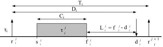
The first to discuss isperiodic tasks. A periodic task is performed on a given frequency. The difference betweenconcreteandnon-concreteperiodic tasks [17], is that concrete periodic tasks are non-concrete periodic tasks extended with a phase. The phase of task i is denoted withΦi and represents the time after timet = 0,
when the periodic task is released.
Aperiodic taskis described withτi, i∈(1,..,n). Each periodic taskτihas arelative deadlineDi, aminimum
periodTi and amaximum computation timeCi. An invocation of a task is called ajob. The kth invocation
of task i is denoted with τik, k∈(1,2,. . . ). Each invocation of τi has its own absolute release time rki and
absolute deadlinedki. Constraints for the absolute values of periodic tasks are:d k
starting timesji andabsolute finishing timefij. Using the absolute finishing time and the absolute deadline, the time a task has left till its deadline can be calculated, called the latenessLji. Thelatenessof a jobτ
j
i, where in general the lateness is negative. Figure 3.1 shows an example, which contains the
i
Figure 3.1: Single periodic non-concrete task with its parameters
Not every task is periodic. There are also tasks that are released at a random moment. Such tasks are called
sporadic tasks. These tasks have the same relative and absolute variables as periodic task. The only different constraint is the one used for the release time. For a sporadic task the (k+1)th invocation happens atrk+1
i ≥
rk i +Ti.
Tasks that have to be executed are grouped in a task set. Anon-concrete periodic task setis denoted withΓ and consists ofnperiodic tasks. Task sets containing concrete periodic tasks are denoted withΩ.
Beside the definitions for tasks and jobs there are also a few functions expressing the behavior of the tasks in the task set. Bellow the utilization, the workload, the processor demand function and the Baruah point will be defined.
Using the basic definitions of tasks, it is possible to calculate the utilization of a task set, as in definition 3.1.1. Note that whenU >1, the schedule is not feasible. There is more load than time to resolve it.
Definition 3.1.1. (Utilization)
TheutilizationU, is the fraction of processor time spent executing the task set. It is defined as:
U =
TheworkloadW(t) of a task set is introduced by Audsley [3]. The equation for W(t) as defined below is used in the feasibility analysis of the EDFI scheduling algorithm.
Definition 3.1.2. (Workload)
The workload offered to the processor by all n tasks, between time 0 and t, is defined by:
W(t) =
This function determines the times a task has been released till time t and multiplies it with the computation time of the task, the work load is the summation of these values for all the tasks. The feasibility algorithms for RMI and DMI scheduling use of an altered version of the workload function. This function calculates the workload only for the j higher priority tasks in the task set. The equation for this function is:
Wj(t) =
The processor demand represents the amount of computation time requested by all jobs that are performed in the period between time 0 and time t. This can be calculated by multiplying the number of deadlines of each task in the period, with the computation time of this task and summing the resulting values for the whole task set. With this equation the feasibility of task sets, scheduled with the EDFI algorithm, can be determined.
3.2. Assumptions
The load that should be resolved by the processor, between t = 0 and t = n, is defined by:
H(t) =
Baruah [28] derived an upper bound for the processor demand function. Using this upper bound a point can be found where this line crosses the processor capacity line, the t =LB line. After this point, the processor
demand will never be larger than the processor can manage. Definition 3.1.4. (Baruah point)
The timeLB limits the period after which the processor demand will always be smaller than the processor
capacity:
The pointLB can be derived from the H(t) function by first defining the upper bound of H(t), also called the
Baruah line:
The point where this upper bound is equal to t can be found by solving the following equation:
t=
For the theory in this report, the assumptions of Jansen [15] are used:
• All tasks in the task set are periodic.
• The schedulers use a highest priority first algorithm.
• The discussed algorithms are non-idling. This means that when there are tasks released and waiting for execution, the processor cannot be idle.
• Scheduling overhead is assumed to be included in the maximum computation time Ciof the task.
• All tasks are independent of each other. There are no precedence constraints, i.e. there is no task that has to wait with executing till another task, referenced with the precedence constraint, has finished.
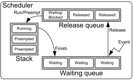
Figure 3.2: Real-time scheduler, with preemption stack, release queue and waiting queue
3.3 General model
In general the transaction system is used in real-time schedulers, see Figure 3.2. This system defines the release and waiting queue and the preemption stack. Tasks are moved from the waiting queue to the release queue when a certain event occurs, for example the event generated by a timer on the start of a new period can release a task. The tasks in the release queue are ordered according to the priority rules of the used scheduling algorithm. The scheduler decides, with the rules of the scheduling algorithm, if the task at the head of the release queue should preempt the task currently on top of the stack. This causes the stack to be arranged according to priority. When a running task finishes, it is placed in the waiting queue.
3.4 Resources
In most operating systems, tasks use resources. Resourcesare functionality available to the whole or parts of the system. Example resources are: specific data, a sensor or a radio for wireless communication. Because resources are shared, read and write access to them has to happen undermutual exclusion. It is assumed that multiple tasks are allowed to read a resource at the same time. Since scheduling algorithms with priorities are used, mutual exclusion can be achieved byinheritanceof the priority from the highest priority task, that will access the resource. First the read and write floor and the inherited deadline are defined. At the end of this section two resource policies will be discussed.
Each resource has aread floorandwrite floor, which contain the highest priority of the tasks that read or write the resource, respectively. The read and write floor are defined by Jansen [15] and slightly modified by Maurer [24]:
Definition 3.4.1. (Read floor Dr R)
DrR=min({∞} ∪ {Di|τi ∈γw(R)}) (3.8)
whereγw(R)is the set of tasks that writes resource R. Definition 3.4.2. (Write floor Dw
R)
Dw
R=min({∞} ∪ {Di|τi∈γw+r(R)}) (3.9)
whereγw+r(R)is the set of tasks that writes and/or reads resource R.
According to Jansen [15], it is possible to define theinherited deadline∆iofτiwith the previous definitions.
3.4. Resources
the set of resources read byτi, is denoted withρri and the set of written resources withρ w
i . With these, the
inherited deadline∆ican defined as:
Definition 3.4.3. (Inherited deadline)
When tasks behave liketransactions, a task only starts when it can use all the required resources without any synchronization. A transaction is run in such a way, that it is run to completion, it should not wait for resource access once it is started. It is however possible that a task is preempted by a higher priority task.
To make sure that a task is not blocked, when it acquires a resources, the deadline inheritance can be used (equation 3.10). This way, if the task can start, it is granted non-blocking use on the shared resources it uses, because it has the highest priority for that resources. Furthermore the priority inheritance can be determined statically. It is known at forehand which resources a task needs, so for each resource the read and write floor can be determined, which can be used to determine the∆iof the tasks.
The resources used by a task are define by ρ. Capital letters are used when write access to a resource is needed, lowercase letters for read access.
ρ : ρwρ|ρrρ|λ
Tasks can also useNested Critical Sections(NCS). An NCS denotes a period, during task executing that certain resources are used. The task will signal the OS when entering or leaving the NCS, this way the OS can arrange mutual exclusive access to the resources during the NCS. Note that, when tasks would be allowed to have only one NCS with the length of the task, the NCS resource policy would behave like the previous explained transaction resource policy.
The NCSs of taskτi are denoted withZi. Bellow two definitions of Jansen [15] are combined to define the
NCS resource policy:
Definition 3.4.4. (Nested Critical Sections)
Taskτihasmicritical sections inZi, whereZi={Zi,0, . . . , Zi,mi}.
• Zi,j= (ρi,j,∆i,j, Si,j) whereρi,j denotes the set of resources used in this critical section,∆i,jis the
inherited priority for this critical section and Si,j denotes the maximum duration that these resources
will be used.
• Critical sections fully overlap or are completely disjoint.
• Zi,0= (∅, Di, Ci), this describes the deadline and the computation time of the task.
The inherited deadline as used in definition 3.4.3 concerns the resources used by a task, while∆i,j in
def-inition 3.4.4 concerns only the resources used by one NCS. Whenρr
i andρwi are redefined as the set of read
or written resources, respectively, for an NCS, definition 3.4.3 can be used. This leaves the entering and the leaving of a critical section undefined:
Definition 3.4.5. (Entering and leaving an NCS)
When taskτienters a nested critical section Zi,j, its∆i drops tomin(∆i,∆i,j). When the NCS is left,∆iis
3
As for transactionsρdefines the used resources for a task. Capital letters or lower case letters are used for write or read access, respectively. The time a task uses a set of resources is given by a float.
ρ → f loat{ρ ρ˜ } |λ
An example concerning the usage of NCSs is given in Figure 3.3. In this Figure taskτ3, from task setΓ1
(Table 3.1), is highlighted. The task starts with its normal delta level of 45. When the task claims resource b and a for writing, its delta level drops to 20 and 10, respectively. These delta levels are equal to the deadlines of the tasksτ2andτ1. The delta level of the task rises to the previous level when an NCS is left.
Table 3.1: Worst-case transaction task setΓ1
Γ1 Di Ti Ci ρi
τ1 10 20 2 2{a}
τ2 20 25 3 3{b}
τ3 45 50 30 5{B 2{A}}
3.5 Task admission and removal
When a task is added to a running task set, first the feasibility of the extended task set has to be analyzed. When the extended task set is feasible, the new task can be released. However, admitting the task may cause the inherited deadlines to change, which may jeopardize the ordering of the preemption stack. For example, when the task with lowest priority has the largest∆, corresponding to the lowest priority, a not shared resource and is at the moment of admission at the bottom of the preemption stack. The new task has the highest priority and writes the resource of the lowest priority task. Adding this new task, would cause the∆-value of the lowest priority task to drop beyond all the deadlines of the tasks on the stack, invalidating the stack ordering. This may cause transitive blocking.
Jansen proposed two methods to insert tasks without disturbing the stack ordering. The first solution is towait for idle time. Since a new task can be added, the utilization of the task set is below 1, so there will be idle time. The second solution is toalter the preemption condition. This solution is outside the scope of this text, details can be found in [15].
3.6. Rate Monotonic with Inheritance
3.6 Rate Monotonic with Inheritance
In 1973 Liu and Layland introduced Rate Monotonic (RM) scheduling [23]. They showed that RM is the
optimalscheduling algorithm, among allfixed priority assignmentscheduling algorithms.
Jansen [15] proposed the extension of Deadline Monotonic (DM) and RM scheduling with Inheritance, called DMI and RMI, respectively. The inheritance is introduced, so the tasks can use resources in a mutual exclusive way. Therefore each taskτiis extended with a∆ias proposed in definition 3.4.3. The used resource policy is
important for the determination of the maximum blocking time, which can be used to determine if task set are feasible.
Definition 3.6.1. (RMI scheduling) The following rules define RMI scheduling:
• The priorities of the tasks are assigned inversely proportional to the periods of the tasks.
• ∀τi ∈ Γ, the Di = Ti.
• Ifτiis in the ready queue, the running taskτrwill be preempted,
if(Ti < Tr) ∨ (Ti < ∆r) = Ti < ∆r
3.6.1 Blocking
When RMI scheduling is used, mutual exclusive access to resources should be granted, as described in section 3.4. Therefore the inherited deadline∆i may contain a higher priority, than theτiactually has. When τi is
running and there is a task in the ready queue with a priority between∆iandTi, this task is blocked.
Definition 3.6.2. (Waiting or blocking, with RMI scheduling)
Ifτiis in the release queue andτris on top of the stack of the processor,τiis waiting if:
Tr≤Ti
τrblocksτi, if:
Tr> Ti∧∆r≤Ti= ∆r≤Ti< Tr
In [15] it is proved that there can be at mostone blockerwhen using the proposed resource policies, with DMI scheduling. Since RMI is a special case of DMI, where the deadlines are equal to the periods, the prove also applies to RMI. With RMI and DMI scheduling, the blocker isrunningorpreemptedat the run time stack. This because the run time stack is fully ordered. This implies, that there will be at most one task on the run time stack which satisfies the blocking condition. Since transitive blocking cannot occur, there will be no deadlocks. It is possible to calculate the maximum blocking load for a task withCB(Ti), as proved in [15]. The function
CB(L)can be defined by:
Definition 3.6.3. (Blocking interval, with RMI scheduling)
The maximum blocking experienced, when using transactions, in an interval with length L is expressed by:
CB(L) = max
j {Cj|∆j ≤L < Tj} (3.11)
The maximum blocking experienced, when using Nested Critical Sections, in an interval with length L is ex-pressed by:
CB(L) = max
Figure 3.4: Critical instant for a lower priority task
3.6.2 Feasibility
The feasibility of a task set can be determined using asufficientalgorithm. This means that, when the task set is determined to be feasible it is feasible. In case it is found to be infeasible by the sufficient algorithm, it can still be determined feasible by the sufficient and necessary feasibility algorithm. If asufficient and necessary
feasibility algorithm determines that a task set is infeasible, it cannot be scheduled by the scheduling algorithm. In general a sufficient feasibility algorithm can be expressed with a short formula, such as theUlub or the
hyperbolic bound, see equation 3.15 and 3.16, respectively. In general a necessary and sufficient feasibility algorithm is a bit more complex.
First a short analysis of the tasks in the task set will be performed. Using this information, a sufficient schedul-ing algorithm for RM will be derived, called the hyperbolic bound. This section ends, with the discussion of the necessary and sufficient scheduling algorithm as introduced by Audsley et al.
Worst-case release times
To determine if a task set is feasible, it is best to check the worst-case situation for the tasks. For that reasons the critical instants are analyzed first. The analysis does not include inheritance, but stays valid when added. Besides that the analysis below is performed with RM scheduling. Analog to this analysis a version for DM scheduling can be derived.
Theorem 1. (Critical instant for a task [23])
A critical instant for any task occurs, if the task is released at the same time t as the higher priority tasks.
Proof : It is first shown that a critical instant occurs when a taskτiis released at the same time as all higher
priority tasks{τj|τj ∈ Γ;j < i; Φi = Φj = 0}. All tasks in the task setΓ are ordered according to their
priority, where the tasksτ1andτnhave the highest and the lowest priority, respectively.
Assume taskτiis released later or at the same time as taskτi−1, soΦi≥Φi−1. According to RMTi> Ti−1,
so one job ofτi will overlap at least two jobs ofτi−1. A job ofτi−1 will delay a job ofτi, whenτi−1is still
executing. To achieve the largest delay, the higher priority task should execute as long as possible while the job ofτistill has to execute. As can be seen for the tasksτ1andτ2in Figure 3.4, the longest delay forτ2can be
achieved whenτ1andτ2are released simultaneously.
Repeating the previous argument for all tasks from the task set, it is shown that the worst-case response for the tasks occurs when they are released at the same time as the higher priority tasks.2
3.6. Rate Monotonic with Inheritance
parameters are:
T1< Tn<2T1
C1=T2−T1
C2=T3−T2
. . . (3.13)
Cn−1=Tn−Tn−1
Cn=T1− n−1
X
i=1
Ci= 2T1−Tn
General feasibility condition
Jansen defined a feasibility condition for a task set scheduled with DMI, derived from the condition of Leung et al [21]. From this theorem the feasibility for a task set scheduled with RMI can be derived, since RMI can be regarded as DMI withDi=Ti.
Theorem 2. (RMI feasibility)
A setΓscheduled with RMI is feasible under blocking, if:
∀i: 1≤i≤n:∃t: 0< t≤Ti:Wi(t) +CB(Di)≤t (3.14)
Proof :Jansen states that the proof is based on two observations. First, when all task are released at t = 0 the load is shifted to the left (theorem 1), which results in the maximal amount of load for i tasks, which can be examined with the Wi(t) function. Furthermore maximum amount of blocking for i tasks can be found with
CB(Di). The second observation is that, if for these i tasks the load can be resolved beforeDi, which is equal
toTi, The worst-case situation can be handled, soΓis feasible.2
Sufficient feasibility algorithms for RM
In [23] the least upper bound for the utilization of a task set scheduled with RM is derived. The least up-per bound is defined by Liu and Layland as in equation 3.15. When n converges to ∞ in this equation, limn→∞Ulub =ln2≈0.69can be found as least upper bound.
Ulub=n(2
1
n −1) (3.15)
The hyperbolic bound is derived in [4] and [5] by Bini et al. They derive a bound for the feasibility of a task set scheduled with RM, which is sharper than the least upper bound in equation 3.15. Therefore the derivation of the hyperbolic bound will be discussed next.
Theorem 3. (Hyperbolic bound)
A task setΓwith n tasks, is schedulable with the RM scheduling algorithm if:
n
Y
i=1
(Ui+ 1)≤2 (3.16)
Proof :Using theorem 1 and equation 3.13, the worst-case scenario can be described. When defining
Ri= Ti+1
Ti and Ui=
Ci
equation 3.13 can be rewritten as follows:
Now it can be seen that:
n−1
Using this, the maximum utilization of the task set can be derived. Note that the search minimizes the maximum utilization among the tasks. The found criterion for feasibility is:
Un≤
from which equation 3.16 can be derived.2
Necessary and sufficient feasibility algorithms for RMI
Anecessary and sufficient feasibility analysis for RM is described by Audsley et al. [2]. Originally this algorithm was described for DM scheduling. The analysis is based on the examination of the longestresponse timeRiin a part of the task set. The response time is the sum of theinterferenceIiand thecomputation time
Ciof taskτi:
Since both sides of the equation contain the variableRi, the smallest value that satisfies equation 3.17 should
be found. A method is proposed with multiple estimations, whereRk
i denotes the kthestimate ofRi. TheIikis
used to define the interference onτiin the interval [0,Rik]:
Iik=
Rifor taskτiis calculated by the following three steps:
1. R0
i = Ci ∧ k = 0.
2. Ik
i for the interval [0,R k
i] is computed by equation 3.18.
3. In caseIik+Ci=Rki, thanR k
i =Riis the worst-case response time.
Else the next estimation can be obtained withRk+1i =Ik
3.7. Deadline Monotonic with Inheritance
In themain iterationof the feasibility algorithm, the subset of the task set is extended with the highest priority taskτi, which is not already in the subset. The response timeRiis the time in which the load of the subset with
taskτi, can be resolved. All tasks are released at the same time to create the worst-case instant, as shown in
theorem 1. When the longest response timeRi, is smaller than the longest deadlineDiin the subset the subset
is feasible. The analysis is extended to support inheritance and blocking. This is done by adding the possible blocking timeBi, of the remaining task set, to the response timeRi of the subset. This gives the following
algorithm:
The Deadline Monotonic (DM) scheduling algorithm was introduced by Leung and Whitehead in 1982 [21]. The DM algorithm drops the constraint of RM, which states that∀τi ∈ Γ : Di = Ti. This introduces the
deadline parameter for each task. Leung and Whitehead also proved theoptimalityof DM, which means that DM schedules all possible task sets which otherstatic priority algorithmscan schedule.
As stated in the previous section, Jansen [15] proposed the extension of RM and DM scheduling with inher-itance, called DMI and RMI, respectively. The definition of a taskτiis therefore extended with the proposed
∆i, from definition 3.4.3.
Definition 3.7.1. (DMI scheduling)
The following rules define the DMI scheduling:
• The priorities of the tasks are assigned inversely proportional to the deadlines of the tasks.
3.7.1 Blocking
The DMI scheduling algorithm is meant to schedule tasks with resources, so it is possible that blocking occurs. Since DMI scheduling is very similar to RMI scheduling, the main part of the blocking computation is similar to section 3.6.1. The major difference is the used priority variable. DMI scheduling uses the deadline as priority and RMI scheduling uses the period. To avoid confusion, the definitions will be restated for DMI, with the correct variables.
Definition 3.7.2. (Waiting or blocking, with DMI scheduling)
Ifτiis in the release queue andτris on top of the stack of the processor,τiis waiting if:
Dr≤Di
τrblocksτi, if:
Dr> Di∧∆r≤Di= ∆r≤Di< Dr
Jansen [15] showed that there can be at mostone blockerwhen using the proposed resource policies from section 3.4, with DMI scheduling. The blocker isrunningorpreemptedon the run time stack, because the run time stack is fully ordered. Since the preemption condition for DMI is used, every task on the run time stack has a smallerDithan the∆jof the task below it on the stack. This implies that there will be at most one task on
the run time stack which satisfies the blocking condition. As for RM, the absence of transitive blocking makes it impossible that deadlocks occur. Because it is not possible that tasks that share resources are at the run time stack at the same time, mutual exclusive access to shared resources is provided.
The maximum blocking load for a task can be found withCB(Di). The functionCB(L)can be defined by:
Definition 3.7.3. (Blocking interval, with DMI scheduling)
The maximum blocking experienced, when using transactions, in an interval with length L can be expressed by:
CB(L) = max
j {Cj|∆j ≤L < Dj} (3.19)
The maximum blocking experienced, when using NCSs, in an interval with length L can be expressed by:
CB(L) = max
j,k {Sj,k|∆j,k≤L < Dj} (3.20)
3.7.2 Feasibility
The feasibility of a task set scheduled with DM scheduling can be determined with a sufficient and a suffi-cient and necessary algorithm. First the general feasibility condition for of a task set scheduled with DMI is introduced. Next a very simple sufficient feasibility algorithm is presented. This subsection concludes with the necessary and sufficient algorithm, which is an optimized version of the sufficient and necessary algorithm in section 3.6.2.
General feasibility condition
Theorem 4. (DMI feasibility (Jansen))
A setΓscheduled with DMI is feasible under blocking, if:
∀i: 1≤i≤n:∃t: 0< t≤Di:Wi(t) +CB(Di)≤t (3.21)
Proof :The proof is as presented in theorem 2. The only difference is the priority parameter, periodDiwhich
3.7. Deadline Monotonic with Inheritance
Sufficient feasibility analysis for DM
From the feasibility test of Lui and Layland in equation 3.15 a sufficient test for DM scheduling can be derived. Since the periodTiof the tasks is increased, the utilization is decreased, which does not affect the feasibility.
A task set scheduled with DM is feasible if the following equation holds:
n
Necessary and sufficient feasibility analysis for DMI
In [15] an optimization of the original algorithm of Audsley et al. 3.6.2 is discussed. The algorithm of Jansen accounts every release of a task once, instead of recalculating the interference in every cycle of the main loop. An altered version of the workload function is used to determine the amount of interference. This function determines the workload for a subset{τ1. . . τj} ⊂Γ, as presented in equation 3.3. Furthermore the algorithm
is extended to account for blocking. The complexity of the optimized feasibility algorithm is ofO(n).
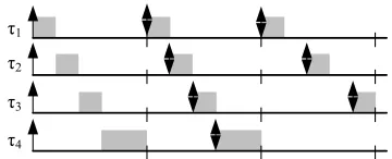
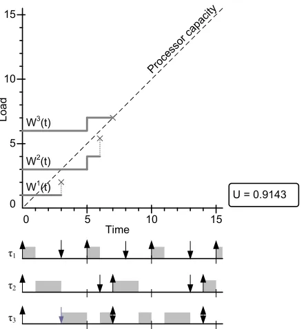
A graphical representation of the algorithm is given in Figure 3.5 for task setΓ2in Table 3.2. The blocking
is visualized with the gray dotted lines, with a cross on top of it. Note that the optimized feasibility algorithm does not start at t = 0 for eachWj(t), but takesWj−1(t)and simply addsC
j to it and continues from the
previous t.
The algorithm presented below has been slightly adjusted, but the core functionality is the same. Each iteration of the main loop extends the examined task set with the highest priority task, which is not already in the examined task set. After every execution of the inner loop, the variable W holds the value ofWj(t).
Table 3.2: Example task setΓ2, using NCS
Figure 3.5: Graphical representation of DMI feasibility analyzes for task setΓ2
3.8 Earliest Deadline First with Inheritance
With the introduction of RM scheduling Liu and Layland introduced deadline driven scheduling [23], nowadays known as Earliest Deadline First (EDF) scheduling. They introduced it as a dynamic priority scheduling algo-rithm, where the priorities are assigned to the task according to the deadlines of their current requests. They also prove that EDF is theoptimalscheduling algorithm among all dynamic priority schedulingalgorithms. This means that every schedule that is found feasible with any dynamic priority scheduling algorithm is feasi-ble with the EDF scheduling algorithm. In [7] Buttazzo repeats the proof of Dertouzos, to show the optimality of EDF. With the proof Buttazzo also shows that EDFminimizes the maximum lateness.
Jansen proposed the extension of EDF with inheritance. The Earliest Deadline First with Inheritance (EDFI) algorithm can be used with the proposed resource policies in section 3.4.
Definition 3.8.1. (EDFI Scheduling) The following rules define EDFI scheduling:
• The priorities of tasks are assigned inversely proportional to the absolute deadlines of the tasks.
• Ifτijis in the ready queue, the running taskτrkwill be preempted, if(d j
i < dkr)∧(Di<∆r).
3.8.1 Blocking
As RMI and DMI, the EDFI scheduling algorithm is also meant to schedule tasks with resources. Therefore the tasks are extended with the proposed∆from definition 3.4.3. This means that it is possible that blocking occurs. In the next definitions the waiting and blocking will be defined.
Definition 3.8.2. (Waiting or blocking, with EDFI scheduling) If the jobτs
r is in the release queue and jobτ j
i is on top of the processor stack,τrsis waiting if:
3.8. Earliest Deadline First with Inheritance
τijblocksτs r, if:
dji > d s
r∧∆i≤Dr
In [15] Jansen shows that there is at mostone blockerwhen using the proposed resource policies 3.4, with EDFI scheduling. The blocker isrunning orpreempted at the processor stack. Since the tasks are allowed to preempt the running instance according to the he EDFI scheduling as defined in 3.8.1, the processor stack is ordered. This implies that there will be at most one task at the processor stack which satisfies the blocking condition, so no transitive blocking and deadlocks will occur. Furthermoremutual exclusiveaccess to shared re-sources is provided when using one of the proposed rere-sources policies, because two tasks which share rere-sources cannot be on the run time stack at the same moment.
Jansen shows that the maximum blocking load for a task can be found withCB(Di). The reasoning behind
the formula is less trivial, as thought. It can be described with the following steps:
1. The interval [t,t+L] is examined to be feasible, including the possible blocking.
2. During feasibility analysis the maximum load is calculated in the interval [0,L], which also has the length L
3. If the load and the blocking do not exceed the processor capacity, it can be concluded that this will not happen for any interval with the length L, anywhere in time.
The blocking interval functionCB(L)for EDFI is equal tot the one defined for DMI in definition 3.7.3.
3.8.2 Feasibility
As with the previous scheduling algorithms, EDFI also hassufficientandnecessary and sufficient feasibility analyses. In 1973 Liu and Layland found a simple feasibility condition, which is necessary and sufficient, for a task set scheduled with EDF scheduling withDi=Ti. They proved that if the utilization is below or equal to
one, so U≤1, the task set is feasible. This analysis does not concern deadlines or resources.
This section starts with the introduction of the general feasibility condition for a task set scheduled with EDFI. Following, a feasibility test for EDF proposed by Devi will be introduced. At the end of this section the necessary and sufficient feasibility test, as introduced by Jansen, will be discussed.
General feasibility condition
Jansen [15] derives the general feasibility condition for EDFI from the condition as defined by Liu and Layland. The condition is:
Definition 3.8.3. (EDFI feasibility)
A scheduleΓis feasible when EDFI scheduling is used, if:
∀L≥0 :H(L) +CB(L)≤L (3.23)
This definition is based on the fact that the processor demand H(L)and the blocking CB(L) should not
exceed the processor capacityL. When for every period the processor demand and the blocking are smaller than the processor capacity, the schedule is feasible.
Sufficient feasibility for EDF and EDFI
Theorem 5. Sufficient feasibility analysis for EDF scheduling A scheduleΓis feasible if:
∀k: 1≤k≤n::
Proof : The algorithm can be proved to be correct, by proving that ifΓis not schedulable by EDF than the previous defined condition is false. This can be done by considering a period [t−1,td), in which a taskτjmisses
its deadline. Taskτk ∈Γis the task with the longest deadline Dk, whereDk ≤(td−t−1). The tasks in the
task set are ordered according their deadlines, where taskτ1is the task with the smallest deadline. The upper
bound of the load that has to be solved by the processor, in the period [t−1,td), can be defined by:
Since taskτj, with j<k, misses its deadline at td, the following can be written:
td−t−1<
Devi also introduces a variation of the feasibility analysis where blocking is considered, under the Protocol Ceiling Policy or the Stack Resource Policy. Since these protocols show similar blocking computations as with EDFI, the equation can be rewritten to:
∀k: 1≤k≤n:: CB·Dk
Necessary and sufficient feasibility for EDFI
3.8. Earliest Deadline First with Inheritance
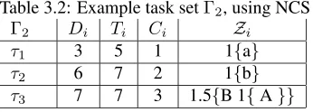
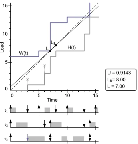
Figure 3.6: Graphical representation of EDFI feasibility analyzes for task setΓ2
that occur. The processor demand function and the blocking are examined at everydeadline, to verify that the feasibility condition holds. When a new task isreleasedthe workload is compared to the processor capacity. All tasks are released at t = 0 to examine the worst-case situation, according to subsection 3.6.2. This introduces the
maximumH(t)
t in the first part of the analysis. When the workload function is equal to the processor capacity
line, point L, all load is resolved and the H(t)
t will never be larger than the processor capacity again. Two
other bounds for the time are the Baruah pointLBand the Least Common Multiple (LCM) of the periods. The
Baruah bound is defined in definition 3.1.4 and shows that the upper bound ofH(t)is always smaller than the processor capacity after the pointLB, which means that the schedule is feasible after that point. When t is
equal to the LCM of the periods of the task set, all tasks are released, because their periods start. This means that the same behavior will show up as when t = 0, so if the schedule was feasible before the LCM it will be after. Furthermore at the LCM of the periods the workload will be equal to the processor demand, which means all load is resolved, another check to determine that the task set is feasible. Figure 3.6 shows a graphical representation of the analysis for the task setΓ2from Table 3.2.
AlgorithmEDFI feasibility analysis
schedulable = unknown; H = 0; // processor demand W = 0; // Workload
LB=
Pn i=1
¡
1−Di
Ti ¢
·Ci
1−U ;
while(schedulable==unknown){ (t,flag,C) = GetNextEvent;
caseflag{ deadline:{
H = H + C;
CB = maxj{Cj|∆j≤t < Dj}
if(H +CB>t){schedulable = no;}
} release:{
if((t >0)∧(W ≤t)){schedulable = yes;} W = W + C;
} }
if((t >0)∧(t≥LB)){schedulable = yes;}
Chapter 4
Earliest Deadline First with Inheritance
and Scaling
When a task setΓis scaled offline, it should still be feasible. Theoffline scalingof a task set means lowering the processor frequencyf before the task set is running, this results in increasing computation times for the tasks. So the main objective of Earliest Deadline First with Inheritance and Scaling (EDFIS) is to determine the maximum amount of scaling of the tasks for which the task set is still feasible.
Scaling can be performed in two ways. The first method is to determine the maximum scaling for each independent task. This introduces an exhaustive search for the optimal frequency distribution. Thesecond methodis to determine the maximum scaling for the whole task set. Because a higher frequency corresponds to an exponentially higher power consumption, it is best to keep the frequencies of the independent tasks as close as possible to the average frequency. Therefore it would be optimal to find the lowest possible frequency for the whole task set.
This section examines the offline scaling of a task set, scheduled with EDFI. First an alternative to scaling all functions used in the feasibility analysis is proposed. The boundaries of the search space for the scaling factor are the point of discussion in section 4.2. This chapter concludes with a method to determine the optimal scaling factor for a task set.
4.1 Scaling the y-axes
When scaling the frequency with a factork <1, theCiof all tasks in a task set are scaled with a factor 1k >1.
When applying the scaledC˜i=Ci·1
k to the workload function 3.2, the processor demand function 3.4 and the
Baruah line function 3.6, the scaling factor can be separated. This is shown in equation 4.1, 4.2 and 4.3. The processor capacityp(t), with slope one (dotted line in Figure 3.6), stays the same. This because the time does not scale, only the load that can be resolved in one unit of time.
Since the factor 1
k can be extracted from all the functions, it is possible to adjust the scale of the y-axis
instead. This results in all the functions staying the same, only the processor capacity line, withp(t) =t, has to be redrawn. Instead of altering the values of the y-axis they can be redefined by stating that they are multiplied with1
k. With this redefined scale the processor capacity line becomesp(t) =k·t. Using the redefined y-axis,
the H(t), W(t) andBL(t)stay the same, they don’t have to be recalculated or redrawn for a new scaling factor.
4.2 Search boundaries
To determine the scaling factor 1
k, the maximal possible utilization of the task set has to be found. When
determining the maximal utilization two cases can be distinguished, the deadlines are equal to the periods, or there is at least one deadline smaller than the corresponding period.
If all tasks in the task set haveDi=Tiand no resources are used the proposition of Liu and Layland can be
used, as mentioned in subsection 3.8.2. They proof that the maximum utilization of the task set is 1. In this case the optimal scaling factor for the task set is 1
k · U = 1, so
1 k =
1 U.
However if the task set has a task withDi < Ti, the analysis is less trivial. This is caused by the load that
has to be resolved at the deadline of the task, which is earlier than the end of the period. This may causes the
H(t)
t to be larger than the utilization U. To determine the maximum H(t)
t the behavior of the task set has to be
examined till a certain timet. This can be done with the functions mentioned in equations 4.1 and 4.2. To find the boundaries in which the maximum H(t)
t can be found, the upper bounds and lower bounds for the
processor demand and workload function are examined. In equation 4.4 the derivation of the lower bound for the processor demand function is shown. The upper bound of the processor demand function, also called the Baruah line function, is already derived in equation 3.6. Equation 4.5 and equation 4.6 shows the derivation of the lower and upper bound for the workload function W(t). Figure 4.1 shows a schematic drawing of these bounds. Note that theslopeof all the bounds is U. It can be seen that the overlap of these areas grows when the difference betweenDiandTiincreases. If the deadlines are equal to the periods,P
n
so the upper bound of H(t) is the lower bound of W(t). Since W(t)≥H(t), the functions can only touch each other in the area or on the line.
H(t) = feasibility algorithm from subsection 3.8.2, three bounds can limit the search space of his verification. The first bound is the point whereall load is resolved, denoted withL. At this point the workload function W(t) touches or intersects thep(t)line, meaning that all load is resolved and that H(t)
t will never be larger than
kagain. The second bound is theLeast Common Multiple(LCM) of all task periods. At this point all tasks are released simultaneously, causing the same behavior to show up as whent= 0. Furthermore the workload function touches the processor demand function when t is equal to the LCM, so it certainly touchedp(t). The third bound is theBaruah point. This is the point where thep(t)function intersects the upper bound of the processor demand functionBL(t). After this pointp(t)is always larger thanBL(t).
4.3. The EDFIS algorithm
Figure 4.1: The bounds for the processor demand function H(t) and the workload function W(t)
functionBL(t). When scaling occurs this function is also scaled with a factork1. Just as with the workload and
the processor demand function this line can be kept the same when the processor capacityp(t)is scaled. To find thescaled Baruah pointBL(t) = k·tshould be solved, as presented in equation 4.7. The found t is the
third boundary, when searching the scaling factor.
k·t=U·t+
The three bounds given on the time, try to prevent the occurrence of an exhaustive search. Nonetheless the scaling causes the utilization to rise to 1. A high utilization causes idle time to be postponed until a later point in time. This means that whenk = U, the workload will only be equal top(t)at the LCM of the periods. Whenk = U bothp(t)andBL(t)have slope U, so no intersection will occur. Note that if k is close to U, the
idle time and the Baruah point are placed far away. A task set can be scaled to a utilization close to U when the deadlines of the tasks get near their periods. Note that the LCM of the task periods can be a very large. For example if two of the task periods are chosen as a prime number, the LCM can be large.
4.3 The EDFIS algorithm
The factorkcan be determined by using the scaled processor capacity line, the workload and the processor de-mand function. With these functions it is possible to determine themax¡H(t)
t
¢
, within the presented boundaries of t. Using this maximum, the scaling is determined byk=max¡H(t)
t
¢ .
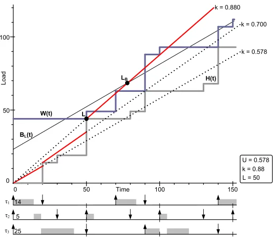
Figure 4.2: Example analysis of task setΓ3
Table 4.1: Example task setΓ3
Γ3 Di Ti Ci
τ1 20 70 14
τ2 30 50 5
τ2 50 90 25
maximum scaling factor within the defined boundaries for the time variablet. The timestamps at which events occur are evaluated. The examined events are the releases and deadlines of tasks. The events are ordered according to their timetand their type, the event with the smallesttis processed first, if two events have the same time and different types, the deadline event is processed first. Deadline events are used to update the processor demand information and release events are used for updating the workload information.
An example of an EDFIS analysis for task setΓ3 in Table 4.1 is shown in Figure 4.2. Initially the scaling
factorkis chosen equal to U, which is 0.578 in the given case. The Baruah lineBL(t)is running parallel to the
initial scaling line, which means that they will never intersect. Note that the Baruah line has slope U and the offsetPn
i=1
³
1−Di
Ti ´
·Ci = 2319 on the y-axis. The two search boundaries left are the LCM of the periods
and the first idle time. The LCM of the periods in this task set is t = 3150 and the first idle time for the scaled task set is found when the workload function is equal to the scaled processor capacityp(t). At t is 20 a deadline event occurs, which introduces a newk= H(t)t = 1420 = 0.7. Note that at t is 20 in Figure 4.2 the old processor capacity line becomes a dotted line and the new line becomes solid. The new scaling factor gives the processor capacity a slope larger than U, so it intersects the Baruah line. The intersection will happen at t = 173.5, which can be calculated using equation 4.7. Continuing the examination of events, the deadline at t is 50 increaseskto
44
50 = 0.88. With the new scaling factor the Baruah pointLBis located at t is 76.5. Furthermore the pointLis
found at t is 50 because the workload function touches the processor demand function and the scaled processor capacity. This means that idle point has passed and the optimal scaling factor has been found.
4.3. The EDFIS algorithm
t with thetimeat which the event occurs, a flag with thetypeof event, either deadline or release, and a C containing themaximum computation timeof the event.
When the event is of typedeadline, the processor demand and the blocking are checked, to see if the scaled processor capacity,t·k, can fulfill the demand. If the processor capacity is to low, the scaling is decreased, so a largerkis chosen. When a larger scaling factor is chosen theBaruah pointis recalculated. Initially the Baruah pointL˜Bof the scaled task set is chosen as infinity, becausekis chosen equal to U, which makes that both lines never intersect.
The workload function is examined when a new job isreleased. When the workload function is smaller than the scaled processor capacity (t·k), all load is resolved by the scaled processor. As with the EDFI feasibility algorithm, no largerk=maxH(t)t can be found after this point.
The last statement of the main loop performs a check, to see iftis larger than the Baruah point. Whentis larger, the optimal scaling is found.
AlgorithmEDFI Scalability analysis
if((schedulable==unknown)∧(t≥L˜B))schedulable=scalable;
Chapter 5
Wireless sensor node
A wireless sensor node is a device equipped with an OS. The hardware platform of the wireless sensor node, as used at the University of Twente, will be discussed in section 5.1. Following the AmbientRT OS will be discussed in section 5.2. This discussion includes the real-time scheduler, the data manager, the modules, the dynamic reconfiguration and the task and data definition in AmbientRT.
5.1 Hardware platform
The sensor node used in this paper is theµnode v2.0 of Ambient Systems, see Figure 5.1. At the moment of writing this is the newest available sensor node. Below the main components of the sensor node will be discussed.
At the hart of the sensor nodes is a Texas Instruments MSP430 microcontroller. This low power microcon-troller has a 16-bit RISC CPU. The MSP430F1611 [30] version of the microconmicrocon-troller is used. This version provides 48 kB flash memory and 10240 B RAM. Much integrated functionality is provided, including:
• 16-bit Timer A with three capture compare registers
• 16-bit Timer B with seven capture compare registers
• 16-bit Hardware multiplier, not integrated in the CPU
• Two Universal Synchronous/Asynchronous Receive/Transmit (USART) interfaces
• Six digital I/O interfaces
• Five power saving modes
• JTAG/debug interface
• Digitally Controlled Oscillator
Theµnode v2.0 is equipped with an EEPROM to provide additional storage space. The used EEPROM is the ST M25P40 [29] 4 Mbit serial flash memory. The flash memory has a Synchronous Peripheral Interface (SPI). It is connected to the digital I/O interfaces of the MSP430.
Figure 5.1: Ambient systemsµnode v2.0
flash memory, this component provides a SPI interface and is connected to one of the digital I/O interfaces of the MSP430.
Beside these main components all nodes have three LEDs. On the edges of the sensor nodes additional digital I/O ports and ADCs are available, to which sensors can be connected. Some sensor nodes are equipped with a MAXIM MAX3319. This component translates the CMOS signals, from the USART interface of the MSP430, to RS232 compatible signals. This makes it possible to communicate with the node by the serial port of a PC.
5.2 AmbientRT
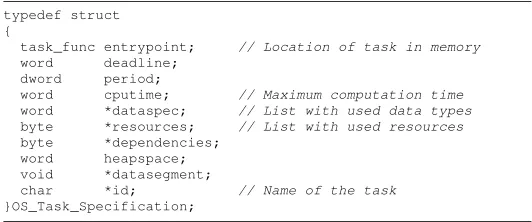
The lightweight OS used on the wireless sensor nodes is AmbientRT, which evolved from the Data-Centric Operating System (DCOS) [12]. AmbientRT is built as a partly platform independent OS. As Hardware Ab-straction Layer(HAL), the OS uses drivers, which provide a general interface to the peripherals. User applica-tions can perform system calls through the funcapplica-tions specified in the AmbientRT library. This library contains general functions like: ”malloc”, ”free” and ”printf”.
The data-centric OS has been developed with four main requirements: real-time scheduling, adata-centric architecture,execution of modulesand the possibility fordynamic reconfiguration. The first two subsections explain the real-time scheduling and the data-centric architecture of AmbientRT. Subsection 5.2.3 explains how AmbientRT executes modules and how it can be reconfigured. The last subsection explains how tasks and data are defined in AmbientRT.