How Symbolic Learning Can Help Statistical Learning
(and vice versa)
Isabelle Tellier
Lattice / Lattice - UMR 8094 Lattice / 1 rue Maurice Arnoux
Lattice / 92120 Montrouge
Yoann Dupont
Lattice / Lattice - UMR 8094 Lattice / 1 rue Maurice Arnoux
Lattice / 92120 Montrouge [email protected]
Abstract
We describe in this paper how different learning strategies can be applied on the same NLP task, namely chunking. The reference corpus is extracted from the French Treebank, the symbolic learning strategy used is grammatical inference and the statistical one is CRFs (Conditional Random Fields). As expected, the sym-bolic approach allows readability but is less effective than the statistical one. We then propose two distinct ways to combine both approaches and show that in both cases they benefit from one another.
1 Introduction
Supervised machine learning approaches, espe-cially when they have access to huge amounts of data, have now extensively proved their effective-ness for a lot of text mining tasks like text classi-fication, sentence annotation and information ex-traction. Most effective learning approaches rely on a theoretical background which is either opti-mization (SVM), statistics (Naive Bayes) or both (HMMs, MaxEnt models, CRFs). But, however effective they may be, the main drawback of these techniques is that they usually do not provide any human-readable model.
There also exists other branches of Machine Learning, referred to as symbolic, whose partic-ularity is to provide a more human-readable out-put. This is the case of decision trees, Inductive Logic Programming (ILP) or Grammatical Infer-ence (GI in the following). The latter is our main interest here. It can be defined as the study of how it is possible to automatically learn a formal grammar or any other device able to represent a language(such as an automaton, a regular expres-sion...) from a sample of (possibly enriched) se-quences known to belong (or not) to this language
(de la Higuera, 2010). This domain is often not very well known due to its roots in theoretical computer science and formal language theory. GI algorithms’ known drawback is their lack of ef-ficiency on real data: they are often time consum-ing, sensitive to errors and do not behave well with large alphabets (for example alphabets containing every word of a natural language).
In this article, we want to give some GI algo-rithms a chance to compete with the state of the art of statistical machine learning approaches. The task we deal with for this purpose ischunking (Ab-ney, 1991) for French, which can be done with hand-made automata (Antoine et al., 2008; Blanc et al., 2010). To our knowledge, trying to auto-matically learn these automatainstead of writing them by hand has never been tested for any lan-guage before. On the other hand, chunking can also be treated as an annotation task (cf. shared task of CoNLL2000) and thus been efficiently pro-cessed by a statistical machine learning approach . The state of the art in this domain are CRFs (Laf-ferty et al., 2001; Sha and Pereira, 2003). Chunk-ing thus seems to be the ideal playground on which both approaches can be fairly compared.
But this comparison is not our only purpose. Our intuition is that both approaches are comple-mentary, as they focus on very distinct properties of the dataset. We also provide in this article two distinct ways to combine them according to dif-ferent purposes. The first one is effectiveness-oriented: it consists in enriching the CRF by automata-based features to improve again its ef-fectiveness. The second strategy is readability-oriented: it consists in analyzing the behavior of an automaton produced by GI thanks to CRF-computed weights which are interpretable with re-spect to this automaton.
The paper is organized as follows. In the first section, we introduce the task of chunking and de-scribe the dataset we have used in all our
ments. The second section is dedicated to gram-matical inference. After a brief review, we focus on thek-RI-algorithms (Angluin, 1982) and pro-vide the best experimental results we could reach with them on the task. In the next section, we apply CRFs (Lafferty et al., 2001) to the same task. As expected, CRFs give far better results than those obtained by GI, at the price of less read-ability. In the last section, we describe and evalu-ate two ways to combine automata and CRFs. The results of both combinations are promising and suggest original trails to associate symbolic and statistical learning.
2 Chunking: the Task and the Data
In this section, we describe the task of chunking as a labeling one and introduce the dataset we used for our experiments. As our purpose is to build a chunker for French, our starting point is the French Treebank (Abeillé et al., 2003).
2.1 The Task
The task ofchunking, also calledshallow parsing consists in identifying elementary (i.e. non recur-sive) syntactic phrases. Chunks are “contiguous and non-recursive lexical units sequences bound to an unique head” (Abney, 1991). Each chunk is characterized by the type (or syntactic category) of its unique head. So, there are as many dif-ferent types of chunks as there are of considered heads. The chunks are thus intimately linked with the part-of-speech (POS in the following) tags as-sociated with the lexical units of the sentences.
Chunking has been the target of the CoNLL shared task in 20001, in which the training set was composed of about 9 000 English sentences taken from the Penn Treebank with two levels of labels: a POS level provided by the Brill tagger and a chunk level. The winners used SVM and “Weighted Probability Distribution Voting”. The same corpus was used to show the effectiveness of CRFs (Sha and Pereira, 2003).
2.2 The Data
The French Treebank (FT in the following) has been built from a collection of sentences ex-tracted from articles of the French newspaper “Le Monde”, published between 1989 and 1993 (Abeillé et al., 2003). The sentences are tokenized
1http://www.cnts.ua.be/conll2000/chunking
(with respect to some multi-word units), lemma-tized, tagged and parsed. There exists multiple versions of the FT, the one we have used is made of about 8 600 XML trees, enriched by syntactic functions which were necessary to identify some chunks. For POS tags, we used the set of 30 morpho-syntactic tags defined by Crabbé and Can-dito (2008).
We consider 7 distinct types of chunks: AP (ad-jectival phrases), AdP (Adverbial phrases), CONJ, NP (noun phrases), PP (prepositional phrase), VP (verbal phrases) and UNKNOWN chunks (usually for those containing foreign words). Punctuation marks between chunks are considered as "out". Unlike Tellier et al. (2012), our CONJ chunk only contains the conjunction token(s) and, as opposed to Paroubek et al. (2006), the epithetic adjectives are always part of the NP containing the noun they qualify, whether they appear before or after this noun. Our AP chunk is thus relatively rare, as it only concerns detached or attribute adjectives (syntactic functions available in the XML trees are needed to identify some of them).
An example chunked sentence in our sense is shown in the following (it means "the depreciation against the dollar has been limited to 2.5%")23: (la/DET dépréciation/NC)N P (par_rapport_au/P dollar/NC)P P (a/V été/VPP limitée/VPP)V P (à/P 2,5/DET%/NC)P P
We extracted from the FT two distinct corpora: •a corpus where every distinct chunk is ex-tracted and labeled with the BIO (Begin/In/Out) convention. Chunks are distributed according to the following proportions: PP: 33,86%, AdP: 7,23%, VP: 17,11%, AP: 2,21%, NP: 32,95%, CONJ: 6,61%, UNKNOWN: 0,03%.
• a corpus where only NPs are labeled, ev-ery other token being considered as out (label O). Recognizing NPs only can be useful for the identi-fication of co-reference chains. This corpus is not a subpart of the previous one, as many PPs include an NP. These "hidden NPs" become visible in the second corpus only, as in the previous example: (la/DET dépréciation/NC)N P par_rapport_au/P (dollar/NC)N P a/V été/VPP limitée/VPP à/P (2,5/DET%/NC)N P
2In this example, NC is the French acronym for CN (com-mon nouns) and VPP is for past participle verbs
3 Grammatical inference
Grammatical Inference (GI) is a domain of re-search which emerged in the 60s and thus has a long history which cannot be easily summed-up. We focus in this section on GI of automata from positive examples. After a brief review, we de-scribe thek-RI algorithms (Angluin, 1982) that we used in our experiments and the results we could reach with them.
3.1 Brief state of the art
GI is the study of how it is possible to automat-ically learn a symbolic device able to represent a language(a formal grammar, an automaton...) from a sample of (possibly enriched) sequences known to belong (or not) to this language (de la Higuera, 2010). When only sequences belong-ing to the language are available, the problem is known as GI from positive examples. This is the case in our context, where no counter-example of any kind is available. This problem is much harder than when negative examples are avail-able, because it is very difficult to avoid over-generalization. Ultimately, if a learning program hypothesizes that the language to be learned is the universal one (Σ∗, whereΣis the alphabet of the language), no positive example can disprove it, even if it over-generalizes.
The first concern of GI was to provide a precise definition of what it means for a program to be able to “learn a language”. The criterion is theoretical and formal, not empirical. A parallel can be drawn with children’s language acquisiton. A child is not “programmed” to learn any specific language, (s)he is able to learn whatever language is spoken in his(her) environment. Similarly, GI programs are required to learnclasses of languages, that is to be able to characterize any member of such a class, when they are provided with examples known to be generated (or not) by this member. The main important “learnability criteria” (also called learn-ing models) are known as “identification in the limit” (Gold, 1967) and “PAC learning” (Valiant, 1984). but we cannot describe them here.
Unfortunately, even for regular languages, the simplest class of the Chomsky hierarchy, those criteria are impossible to fulfill with positive ex-amples only: there is no algorithm able to learn from positive examples the whole class of regu-lar languages satisfying these criteria (Gold, 1967; Kearns and Vazirani, 1994). Researchers have
thus tried to identify learnable smaller or trans-verse classes in Chomsky’s hierarchy (Angluin, 1980).k-reversible languages (Angluin, 1982) are such classes, and were the starting point of our ex-periments. Many other learnable subclasses have been described and studied, for example in Gar-cia and Vidal (1990; Denis et al. (2002; Kanazawa (1998; Koshiba et al. (2000; Yokomori (2003).
Other advances in the domain concern the learn-ability of devices integrating probabilities, such as probabilistic automata and their links with HMMs (Thollard et al., 2000; Dupont et al., 2005). In par-allel, challenges4allowed to test the effectiveness of the proposed algorithms when confronted with real data.
3.2 k-RI Algorithm
In this section, we describe the GI algorithms used for our experiments. They were applied to try and learn a chunk-specific automaton from the positive sequences of POS tags extracted from the train-ing part of the dataset. GI algorithms from pos-itive examples seem adapted to this problem, as the considered alphabet is limited (30 distinct tags at most) and each distinct kind of chunk can be de-scribed by a relatively limited number of syntactic constructions.
k-Reversible Inference (k-RI) algorithm (An-gluin, 1982) has the property of identifying in the limit anyk-reversible language, for any fixedk∈
N. The class ofk-reversible languages is a
sub-class of regular languages, and its members can thus be represented by Deterministic Finite State Automata (DFA). An automaton isk-reversible if it is deterministic and its mirror 5 is determinis-tic with a look-ahead of k. When k = 0, a 0 -reversible language can be represented by a DFA whose mirror is also deterministic, the algorithm being called Zero Reversible (ZR). Ifk1< k2, the
class ofk1-reversible languages is stricty included
in the one ofk2-reversible lanugages.
Given a set of positive sequences S, the first step of k-RI is to build PTA(S), the Prefix Tree Ac-ceptor of S. PTA(S) is a tree-shaped DFA, and it has the property of being the smallest tree-shaped DFA recognizing exactly the language defined by S. The root of PTA(S) is its initial state. The search
4The most recent ones were Stamina (http://stamina.chefbe.net) and Zulu (http://labh-curien.univ-st-etienne.fr/zulu)
Step 1 : PTA(S)
Step 2 : final states of PTA(S) are merged
Step 1 : mirror of PTA(S)
Step 3 : q1 and q2 are
merged
Figure 1: Step by step demo of ZR
space of a GI algorithm for a given training set S of positive examples is a lattice whose bottom el-ement is PTA(S) and top elel-ement is the universal language built from the alphabet of the examples (Dupont et al., 1994). Most GI algorithms start by building the PTA of the set of available pos-itive examples, then try to generalize the recog-nized language by merging some of the states of this automaton. k-RI, detailled below, works ac-cordingly. The merging operation here is deter-ministic, as it propagates recursively through the automaton to preserve determinism.
Algorithmk-RI
In: S : a set of (positive) sequences,k: natural;
Out: A : ak-reversible automaton;
begin
A := PTA(S);
whilenot(Ak-reversible)do
// let N1 and N2 be two nodes // violatingk-reversibility of A. Deterministic_Merge(A, N1, N2);
end while; returnA;
endk-RI;
In Figure 1, we illustrate how ZR be-haves with the following set of positive ex-amples of sequences of POS tags: S =
{DET N C, DET ADJ N C}. On this example, we see that ZR already generalizes PTA(S) to output an automaton recognizing the language defined by the regular expression: DET ADJ∗ N C. This generalization is lin-guistically relevant. But if we add to the previ-ous positive sample the sequence made of N C alone, ZR will output an automaton recognizing the language{DET|ADJ}∗N C, which is a more doubtful generalization.
3.3 GI Experience Results on NP Chunking
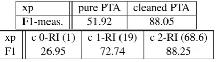
We applied k-RI for different values of k (k = 0, k= 1, k= 2) on POS tags sequences matching NP chunks in the corpus of NP chunks only. This task is the one for which GI is the most appro-priate. It is also possible to learn chunk-specific automata on the other corpus, but the application of multiple automata on new data pose a frontier covering problem. Therefore, we only use them in combination with a statistical model, in section 5. ZR is really sensitive to the available data. A single incorrect sequence can force many states to merge. It was often the case with our dataset, where outliers or tagging errors are not absent. But some erroneous examples can be easily detected: for example, sequences of tags for a special kind on chunk which do not even contain any possi-ble head tag of this chunk can be removed. Other cleaning strategies have been tried. Removing any sequence that occurs less than a fixed proportion was the most effective. Some information loss was nevertheless inevitable as there are heads that were rare (some clitics, for example).
Our experiments were made following a 5-fold cross-validation protocol. A learnt automaton is used as a regular expression on every new se-quence of POS tags, looking for the smallest (resp. longest) matches (sm resp. lm). The correctness of a chunk is evaluated in a strict sense, i.e. it is cor-rect if and only if both frontiers are corcor-rect. The precision, recall and F1-measure of NP-chunks are computed without taking into account O labels. Table 1 contains various F-measures that we man-aged to obtain by GI only on NP chunking, with a longest match strategy. Cleaned (c) versions are obtained by deleting every POS sequence that ap-peared strictly less than 0.01%. Values between parentheses are the medium sizes (in numbers of states) of the 5 automata sizes. PTA versions, whose performances are sometimes good, can be seen as “learning by heart” devices, as they are not generalized. Automata of size 1 are those, proba-bly overgeneralized, that recognize the universal language of POS tags present at least once in NP chunks.k≥2is necessary to obtain an automaton behaving better than the cleaned PTA.
4 Statistical learning for annotation
xp pure PTA cleaned PTA F1-meas. 51.92 88.05 xp c 0-RI (1) c 1-RI (19) c 2-RI (68.6)
F1 26.95 72.74 88.25
Table 1: GI results for NP chunking
recall how some HMMs can be "transformed" into a CRF, as it will be useful further.
4.1 Conditional Random Fields and HMMs
CRFs have been introduced by Lafferty et al. (2001). They belong to the family of graphical models. When the graph is linear (which is most often the case), the probability distribution that the annotation sequence y is associated with the input sequencexis expressed by:
p(y|x) = 1
Z(x) Y
t
exp XK
k=1
λkfk(t, yt, yt−1, x)
WhereZ(x) is a normalization factor depending onx. This computation is based onK featuresfk (usually binary functions), provided by the user. The featurefkis activated (i.e.fk(t, yt, yt−1, x) = 1) if a configuration occurring at the current po-sition t in the sequence, concerning yt, yt−1 (i.
e. the values of the annotation at the positionst and t −1) and x is observed. Each feature fk is associated with a weight λk which are the pa-rameters of the model, to be estimated during the learning step. To define large enough a set of fea-tures, softwares implementing CRFs help users: they usually only require to provide feature tem-plateswhich are automatically instanciated into as many features as there are positions in the training data where they can apply. The most current ef-ficient implementation of linear CRFs is Wapiti6, which uses a L1 penalization allowing to select the best features during the learning step (Lavergne et al., 2010). It is the software we have used.
CRFs have been applied with great success to various annotation tasks, among which POS label-ing (Lafferty et al., 2001), named entity recogni-tion (McCallum and Li, 2003), chunking (Sha and Pereira, 2003) and even full parsing (Finkel et al., 2008; Tsuruoka et al., 2009). Their main draw-back is that they appear as "black boxes". A CRF model is simply characterized by a list of weighted
6http://wapiti.limsi.fr/
features but it is not unusual that it contains thou-sands, even millions of such features. The result is therefore not easy to interpret.
HMMs, which were the previous state of the art for annotation tasks, have the merit to be more un-derstandable. However, every discrete HMM can be “transformed” into a CRF model defining ex-actly the same probability distribution (Sutton and McCallum, 2006; Tellier and Tommasi, 2011). To do this, you have to define two families of features: • features of the form f(yt, xt) associating an individual labelytwith an individual inputxt: they correspond to the statesytof the HMM where xtcan be emitted;
•features of the formf(yt−1, yt) correspond-ing to the transitions of the HMM linkcorrespond-ing the states yt−1 andyt.
If θ is a probability of emission or of transi-tion of the HMM, then chooseλ =log(θ)as the weight of the corresponding feature in the CRF. The computation ofp(y|x)then writes exactly the same in both cases. Discrete HMMs can thus been seen as a special case of CRFs. But CRFs are more general because they allow features to be more general than those used in this transforma-tion. This transformation inspired us to use CRFs to analyse a discrete automaton learned by GI. This will be studied in section 5. Before, we pro-vide the learning results obtained by using a CRF on our data.
4.2 Experimental Results
Tables 2 shows the feature templates and results obtained by using CRFs alone on both chunking tasks. For these experiments, we also followed a 5-fold cross-validation protocol and evaluated the chunks in a strict sense. For the complete chunking task, we computed both the micro-average of F-measures (i.e. the average of the F-measures of every kind of chunk weighted by their frequencies) and their macro-average (i.e. without any weight). As expected, CRFs provide excellent results. It is to be noted that they use words in their features along with POS tags, while GI algorithms have only access to the latter.
5 Combinations
Feat Type Window Word Unigram [-2..1] POS Bigram [-2..1] chunking Complete NP only
micro 97.53 N/A
macro 90.49 N/A
F1-measure N/A 96.43
Table 2: Template and obtained results with CRFs for each task
but not very effective programs, whereas it is the contrary for statistical learning. In this section, we want to combine both strategies. There are two different possible viewpoints for this combination: • if we stand from the viewpoint of effec-tiveness, we will favor statistical leaning. But the automata provided by our GI algorithms capture long-distance relationships between POS tags that could be useful for a CRF. So, in this case, our combination strategy will consist in integrating the output provided by the automata into the features of the CRF as an external resource.
• if we stand from the viewpoint of read-ability, we will favor the automata produced by GI. As evoked in 4.1, it is possible to simulate a HMM (and, similarly, an automaton) with CRF’s features. We will show that it is also possible to evaluate the states and transitions of an automa-ton with CRF-computed weights associated to the features that represent them in a CRF, suggesting ways to improve it.
5.1 Enriching a CRF by automata-based features
We attack here both types of chunking. The first combination consists in considering the automata as independent annotation tools, as in Constant and Tellier (2012). In the case of complete chunk-ing, we applied GI on each distinct type of chunk, leading to as many automata as there are types of chunks. Each chunk-specific automaton provides an independent BIO tagging, as shown in Table 3. Therefore, there are as many new attributes as there are types of chunks in our data.
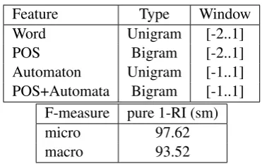
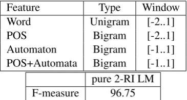
First tables in Tables 4 and 5 give the templates used to obtain the best results for the complete chunking, and similarly for the first one of Table 6 for the NP-chunks only. The lines “Automaton” take into account the output of each automaton independently, whereas “POS+Automata”
repre-word POS NP VP PP ... correct label
la DET B O O ... B-NP
dépréciation NC I O O ... I-NP
par_rapport_au P O O B ... B-PP
dollar NC B O I ... I-PP
a V O B O ... B-VP
été VPP O I O ... I-VP
limitée VPP O I O ... I-VP
à P O O B ... B-PP
2,5 DET B O I ... I-PP
% NC I O I ... I-PP
Table 3: Dataset Enriched by the Output of the chunk-specific Automata
sents the concatenation of POS columns along with the output of every single automaton.
Matching results are given in the other tables. They show that attributes taken from automata al-low to significantly improve the results of CRFs. It is even more obvious for the macro-average, the one that gives equal importance to every chunk. This means that the information brought by the automata mostly improve the recognition of rare chunks. In the experiment leading to the best macro-average, the best improvements are the fol-lowing: the F1-measure of UNKNOWN goes from 41.67 to 61.22, the one of AP from 96.78 to 97.44 and the one of AdP from 98.72 to 98.92.
Feature Type Window Word Unigram [-2..1] POS Bigram [-2..1] Automaton Bigram [-2..1]
F-measure pure 1-RI (lm)
micro 97.66
macro 92.22
Table 4: Best micro-aver. for complete chunking
Feature Type Window
Word Unigram [-2..1]
POS Bigram [-2..1]
Automaton Unigram [-1..1] POS+Automata Bigram [-1..1]
F-measure pure 1-RI (sm)
micro 97.62
macro 93.52
Feature Type Window Word Unigram [-2..1]
POS Bigram [-2..1]
Automaton Bigram [-1..1] POS+Automata Bigram [-1..1]
pure 2-RI LM F-measure 96.75
Table 6: Best F-measure for NP chunking
Figure 2: Unitex-generated automaton
5.2 Evaluating an automaton by CRF-computed weights
This time, we want to preserve the structure of the automata output by our GI strategies, but we use a CRF to evaluate some of their properties. We could build weighted automata, the way it is pro-posed by Roark and Saraclar (2004). Instead, we just propose a CRF-based diagnosis of a purely symbolic device. To illustrate our approach, we consider the NP-only chunking task, because only one automaton is to be considered. Our proposi-tion is also easier to understand by representing automata in the alternative way of Figure 2 (rep-resenting the same automaton as the final one of Figure 1). This representation, which is favored in softwares like Unitex7, has the advantage of dis-playing tags and transitions between tags as two distinct objects. To build a CRF based on such an automaton, we consider the BIO labeling effect of this automaton, as in section 5.1
Now, inspired by the relationship between dis-crete HMMs and CRFs (cf. section 4.1), we choose features which can be interpretable rela-tively to the automaton. We thus restrict ourselves to only two feature-templates:
•the unary feature-template only takes into account the current correct BIO NP-label together with the current POS tag and the current BIO la-bel predicted by the automaton at the same po-sition. Each POS tag matches one (or multiple) states of the automaton. If both BIO labels match for a given POS tag, then the features generated by this template express the correctness of the au-tomaton at this position; if they are different they
7http://www-igm.univ-mlv.fr/ unitex/
express its incorrectness
• the bigram feature-template only takes into account the current correct couple of BIO NP-labels together with the corresponding cou-ple of consecutive POS tags as well as the corre-sponding couple of BIO automaton-predicted la-bels. The couples of consecutive POS tags char-acterize transitions of the automata. If the corre-sponding two couples of BIO labels coincide, it means that the automaton has correctly treated this transition, otherwise it has not.
Note that words, which do not appear in au-tomata, are neither not taken into account in the feature-templates. The generated features have a constrained form to match the automaton struc-ture. All of them are interpretable with respect to this automaton, as we will see now.
Table 7 is a confusion matrix comparing “automata-generated” BIO labels (AL) with the corresponding correct BIO label (CL), for a given POS tag. We can build as many such tables as there are distinct POS tags in NP chunks (the DET tag, in our example), each cell corresponding to an unigram feature. The cells of 7 are filled with the weights computed by the CRF for these fea-tures, where the colors display how they can be interpreted with respect to the initial automaton. As expected, weights on the diagonal, meaning a correct tagging, are positive and greater than those outside it, meaning a tagging error.
AL \CL B I O
B 1.66 -4.05 -0.84 I -0.44 0.46 -2.51 O -1.45 -1.02 -0.17
Table 7: Confusion matrix for DET tag (2-RI, Ta-ble 1)
Where each cell can be interpreted as follows: •no style : both outputs are identical.
•italic: premature chunk beginning. •bold: missed chunk beginning. •italic: untimely chunk continuation. •bold: premature chunk ending.
transi-Exp. baseline (GI) 0-RI 1-RI 2-RI chunk 88.25 93.00 93.07 93.08
Table 8: Labeling results of the CRFs based on the best automata for NP-chunking
tion has 9 lines and 9 columns, because there are
9 = 3∗3distinct possible couples of BIO labels. Each cell corresponds to a bigram feature and is interpretable with respect to the transitions of the NP automaton. Each cell can thus also be filled with the weights associated to the corresponding feature by the CRF model.
The weights associated to the features in a CRF characterize theirdiscriminative power. They are more relevant than the simple occurrence counts of how many times the features are satisfied in the training dataset. The content of diagonal cells can thus be seen as a measure of the effectiveness of the decision taken by the automaton at a state (resp. a transition) whereas the content of the other cells can be seen as the gain (or loss) taken by us-ing an alternative decision at any time, durus-ing the labeling process. So, the whole set of confusion matrixes can be seen as a very precise evaluation of the relevance of the automaton.
Table 8 recalls the result of the best “pure GI” NP-automaton of section 3.3 and gives the label-ing result of the CRFs defined as described above on the best automata output by k-RI, for each value of k. We see that the CRFs significantly improve the efficiency of the best automata, but are not as effective as a CRF using more attributes and features. This results can be interpreted as fol-lows: it is sometimes beneficial to take labeling decisions which are not those of the automata. We still haven’t taken the time to analyze the various confusion matrices produced by our CRFs in these cases, but we believe that they give very interest-ing indications about how, where and why the au-tomata on which the features are based made right vs. wrong predictions, and possibly correct them.
6 Conclusion and perspectives
In this paper, we have applied two distinct ma-chine learning approaches on the same dataset and proposed two distinct ways to combine them.
About GI alone, it is possible that other algo-rithms would give better results than k-RI, such as those of Garcia and Vidal (1990; Denis et al. (2002). The choice of a greater value of kcould
also improve our results, but at the cost of a greater time complexity8. More generally, it should be necessary be to define a learnable language class to which chunks are likely to belong. This would allow to define specific GI algorithms for this task, in which for example linguistic knowledge could be used to “control” state merges .
But the most original part of our work concerns CRFs and automata combinations. It is to be noted that they can both be applied to hand-made au-tomata, likely to be more linguistically relevant than those obtained by GI. We focused here on automata produced by machine learning to show that, even without any linguistic expertise, it is possible to combine symbolic and statistical mod-els. The intuition behind this work is that both machine learning techniques have complementary properties and should benefit from one another. CRFs are based on a huge number of weighted local configurations. It is theoretically possible to express in their features complex long-distance properties of the initial sequencex. In practice, it is rarely done. GI on the contrary applies to se-quences and is able to provide a generalization of a set of sequences. It has already been observed that CRFs benefit from features expressing more general properties than simple local configurations (Pu et al., 2010). Our intuition was that GI could provide such useful generalizations. The obtained results confirm this intuition. It is also interesting to see that symbolic models enhance the treatment of rare cases, on which statistical models do not behave well.
CRF-generated confusion matrices for the anal-ysis of an automaton still need to be further in-vestigated. How to better interpret or take advan-tage of them is of particular interest. Some of the cells of these matrices are empty, either because the corresponding feature has not been observed in the training set or because it has been discarded by Wapiti during the learning step because of the penalty. It should be possible, thanks to this in-formation, to modify the automaton on which the CRF is based by removing/adding states or tran-sitions according to the diagnosis of the confusion matrices. A CRF-directed GI strategy still needs to be defined. This kind of GI challenge could also benefit from existing learning algorithms targeting probabilistic automata (Thollard et al., 2000).
8k-RI time complexity is of|Σ|k|Q|k+3where|Q|is the
[Sutton and McCallum2006] Charles Sutton and An-drew McCallum, 2006. Introduction to Statisti-cal Relational Learning, chapter An Introduction to Conditional Random Fields for Relational Learning. MIT Press, lise getoor and ben taskar edition.
[Tellier and Tommasi2011] Isabelle Tellier and Marc Tommasi. 2011. Champs Markoviens Condi-tionnels pour l’extraction d’information. In Eric Gaussier and François Yvon, editors,Modèles prob-abilistes pour l’accès à l’information textuelle. Her-mès.
[Tellier et al.2012] I. Tellier, D. Duchier, I. Eshkol, A. Courmet, and M. Martinet. 2012. Apprentissage automatique d’un chunker pour le français. InActes de TALN’12, papier court (poster).
[Thollard et al.2000] Franck Thollard, Pierre Dupont, and Colin de la Higuera. 2000. Probabilistic DFA inference using Kullback-Leibler divergence and minimality. InProc. 17th International Conf. on Machine Learning, pages 975–982. Morgan Kauf-mann.
[Tsuruoka et al.2009] Y. Tsuruoka, J. Tsujii, and S. Ananiadou. 2009. Fast full parsing by linear-chain conditional random fields. InProceedings of EACL 2009, pages 790–798.
[Valiant1984] L.G. Valiant. 1984. A theory of the learnable. Commun. ACM, 27(11):1134–1142, November.