High WSD accuracy using Naive Bayesian
classifier with rich features
Cuong Anh Le andAkira Shimazu
School of Information Science, Japan Advanced Institute of Science and Technology (JAIST) 1-1, Asahidai, Tatsunokuchi, 923-1292, Ishikawa
, Japan
{cuonganh,shimazu}@jaist.ac.jp
Abstract
Word Sense Disambiguation (WSD) is the task of choosing the right sense of an ambiguous word given a context. Using Naive Bayesian (NB) classifiers is known as one of the best methods for supervised approaches for WSD (Mooney, 1996; Pedersen, 2000), and this model usually uses only a topic context represented by unordered words in a large context. In this paper, we show that by adding more rich knowledge, represented by ordered words in a local context and collocations, the NB classifier can achieve higher accuracy in comparison with the best previously published results. The features were chosen using a forward sequential selection algorithm. Our experiments obtained 92.3% accuracy for four common test words (interest, line, hard, serve). We also tested on a large dataset, the DSO corpus, and obtained accuracies of 66.4% for verbs and 72.7% for nouns.
1.
Introduction
WSD is always a difficult and important task in natural language processing. Its task is to determine the most appropriate sense for an ambiguous word given a context. Approaches for this work include supervised learning, unsupervised learning, and combinations of them. Except for the expense involved in building labeled datasets, supervised based methods generally give results with higher precision. Many supervised learning algorithms have been applied, such as Bayesian learning, Exemplar-Based learning, Decision Trees, Decision Lists, and Neural Networks. Despite their simplicity, NB methods are still effective when applied to WSD (Mooney, 1996; Pedersen, 2000).
Before presenting the previous related studies and describing our approach, we need to define some terms that are used throughout in this paper. These are topic context, local context, and
collocation. The first kind of information, which is always used for determining the senses of a word,
is the topic context represented by a bag of surrounding words in a large context of the ambiguous word. The other informative resource is collocation. There are various definitions of collocation, and for our approach we define collocation as a sequence of words including the ambiguous word. Several studies, such as Leacock and Chodorow (1998), used local context for disambiguating word senses. Like them, we define local context as the words (or tags of words) assigned with their position in relation to the ambiguous word in a local context. For example, suppose that we have a context of the ambiguous word interest as follows:
“yields on money-market mutual funds continued to slide, amid signs that portfolio managers expect further declines in interest rates.”
Then the topic context includes the words: yields, money-market, mutual, funds, continued, . . .;
Collocations include the expressions: interest rates, declines in interest, in interest rates, further declines in interest rate ,. . .; Local context is represented by the pairs: (declines,-2), (in,-1), (rates,1),
(further, -3), . . .
Note that words in collocations and local contexts can be replaced by their part-of-speech tags, and then we will have new features. We also use other terms in the same meaning: unordered words as surrounding words, and ordered words as the words assigned with their positions.
classifier itself as an evaluation function to find the most appropriate sizes for the windows of features in local context and for collocation lengths. Second, from the initially selected features, we used the Forward Sequential Selection (FSS) algorithm presented in Domingos (1997) for extracting the best subset of features. In FSS, the searching process starts with an empty set. First, feature subsets with only one feature are evaluated and the best feature (f*) is selected. Then, two feature combinations of f* with the other features are tested and the best subset is selected. The search goes on by adding one
more feature to the subset at each step until we do not get any more performance improvement for the system.
Note that we do not use the feature selection on the whole features because of the big set of features (some thousands of features). We prefer the objective of selecting subsets based upon the kinds of features to that of extracting the best features from the whole. We followed the wrapper approach and used the NB classifier itself as the evaluation function.
Therefore, feature selection was divided into two steps as follows:
Step 1: Set 4 as the maximum size for both local context and collocation length. Based on the results obtained by testing on the four words using a 10-fold cross validation, find the most appropriate sizes for local context and collocation length.
Step 2:
Function Automatic Feature Selection
Generate a pool of feature sets PF = {F1, F2, F3, F4, F5}
Initialize the set of selected feature set SF = Ø
Let BestEval = 0
Repeat
Let BestF = None
For eachF in PF and not in SF
Let SF’ = SF∪ {F}
IfEval(SF’) > BestEval
Then
Let BestF = F
Let BestEval = Eval(SF’)
IfBestF≠None
Then Let SF = SF∪ {BestF}
UntilBestF = None or SF = PF
ReturnSF
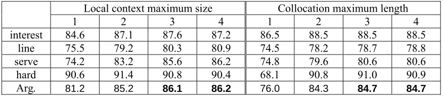
At the first step of the feature selection algorithm, we used the feature set F2 as test data to get the
best local context window size, and used set F4 to get the best collocation size. We implemented the
algorithm with the maximum sizes of both local context and collocation runs from 1 to 4, and obtained the results shown in Table 1.
Local context maximum size Collocation maximum length
1 2 3 4 1 2 3 4
interest 84.6 87.1 87.6 87.2 86.5 88.5 88.5 88.5
line 75.5 79.2 80.3 80.9 74.5 78.2 78.7 78.8
serve 74.2 83.2 85.6 86.2 74.8 79.6 80.6 80.6
hard 90.6 91.4 90.8 90.4 68.1 90.8 91.0 90.9
Arg. 81.2 85.2 86.1 86.2 76.0 84.3 84.7 84.7
From those results, we can see that there are no significant differences in obtained accuracies between using size 4 and size 3 for both local context and collocation. For sizes 1 and 2, the accuracies are much lower. Therefore, we chose 3 as the most appropriate size for both local context window and collocation length.
At the second step of the algorithm, the average of results obtained from testing on the four words using a 10-fold cross validation is used as the evaluation function Eval(SF) for the feature set SF.
In the algorithm, we used only the content words in topic context. This means that we removed the words with tags including determiners, articles, pronouns, auxiliary verbs, prepositions, adverbs, and numbers. Unlike some other studies, we used all terms (unordered words, ordered words, collocations) without requiring that their frequencies be greater than a determined threshold. This was because from our experimental results, we found that the NB classifier will perform better if it combines evidence from all of the features rather than making a decision by testing only a subset of features with highly frequencies.
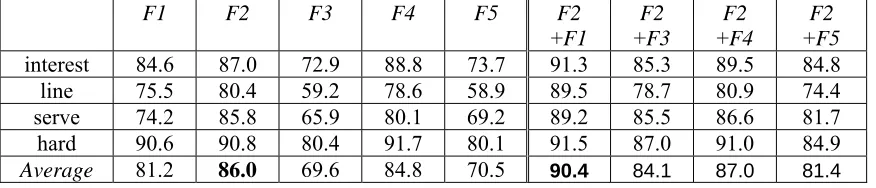
The results obtained in step 2 of the algorithm are shown in the tables below. Table 2 shows the results achieved at the first and second iterated steps; at the first step, F2 is proved to be the best
information for determining word senses, and the combination of F2 and F1 is proved to be the best at
the second iteration. Table 3 shows the results of the third and the fourth iterations, and we learn that the combination of three features sets, F2, F1, and F4, will give the highest accuracy, and the next
iteration decreases the accuracy.
F1 F2 F3 F4 F5 F2
+F1
F2
+F3
F2
+F4
F2
+F5
interest 84.6 87.0 72.9 88.8 73.7 91.3 85.3 89.5 84.8
line 75.5 80.4 59.2 78.6 58.9 89.5 78.7 80.9 74.4
serve 74.2 85.8 65.9 80.1 69.2 89.2 85.5 86.6 81.7
hard 90.6 90.8 80.4 91.7 80.1 91.5 87.0 91.0 84.9
Average 81.2 86.0 69.6 84.8 70.5 90.4 84.1 87.0 81.4
Table 2. Results at the first and second iterated steps
Table 3. Results at the third and fourth iterated steps
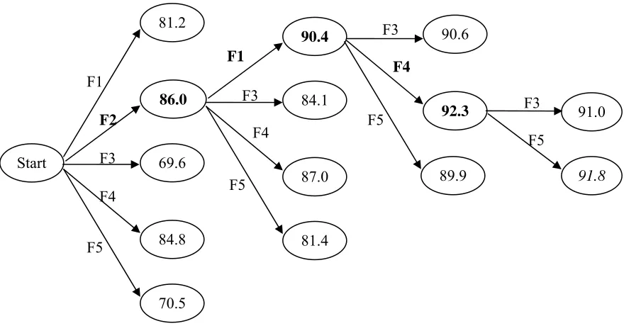
In summary, after running this function, we achieved {F1, F2, F4} as the best subset of features.
In comparison with other studies, Leacock and Chodorow (1998) lacked collocations, Ng and Lee (1996) lacked local context, and Escudero (2000a, 200b) used local context and collocations with smaller sizes. In addition, all of them used part-of-speech information, and Ng and Lee (1996) added syntactical information to their features.
Figure 1 shows intuitively the results of the feature selection algorithm at step 2. First, feature F2
is selected, next feature F1 is selected, then feature F4 is selected, and at the final iteration, no more
features should be selected.
F2+F1
+F3
F2+F1
+F4
F2+F1
+F5
F2+F1+F4
+F3
F2+F1+F4
+F5
interest 91.2 93.2 91.3 92.9 92.4
line 90.1 91.8 89.3 90.3 91.5
serve 90.2 91.4 90.0 90.2 91.7
hard 90.9 92.6 89.0 90.7 91.5
Average 90.6 92.3 89.9 91.0 91.8
4.
Experiments
In order to widely compare this method to others, we tested on four words which are used in numerous comparative studies of word sense disambiguation methodologies such as Pedersen (2000), Ng and Lee (1996), Bruce & Wiebe (1994), and Leacock and Chodorow (1998).
Bruce &
Wiebe, (1994) (%)
Mooney, (1996)
(%)
Ng & Lee, (1996)
(%)
Leacock& Chodorow,
(1998) (%)
Pedersen, (2000)
(%)
Our method
(%)
interest 78 - 87 - 89 93.2
line - 72 - 84 88 91.8
serve - - - 83 - 91.4
hard - - - 83 - 92.6
Average - - - - - 92.3
Table 4. Comparison with previous results
These words include interest, line, serve, and hard. We obtained those data from Pedersen’s
homepage (1). There are 2369 instances of interest with 6 senses, 4143 instances of line with 6 senses, 4378 instances of serve with 4 senses, and 4342 instances of hard with 3 senses. Note, however, that
some of these studies did not use all four words in their experiments. We used a 10-fold cross validation for our experiment. Table 4 shows our results are much more accurate than the previous results.
5.
Test on large data
For evaluating on a large dataset, we tested the DSO corpus published in Ng and Lee (1996), which contains 192,800 semantically annotated occurrences of 121 nouns and 70 verbs corresponding to most frequently used and ambiguous English words. This corpus is now available in the Linguistic
1 http://www.d.umn.edu/~tpederse/data.html Start
86.0
69.6
84.8
70.5 F1
F2
F3
F4
F5
84.1
87.0
81.4 F3
F5 F4
92.3
89.9
F5 91.0
91.8
F3
F5
Data Consortium (LDC)2. It contains sentences without part-of-speech tags, and in each sentence the ambiguous word is labeled with a sense. We did not use a part-of-speech tagger for this corpus and so for topic context we used only some stopped words including articles, determiners, pronouns, and auxiliary verbs. The obtained accuracies are 66.4% for verbs and 72.7% for nouns. We also experimented on DSO corpus using only topic context (feature F1) for comparison and achieved an average accuracy of 63.1%.
Ng and Lee (1996) (Exemplar-based)
Escudero et al. (2000b) (LazyBoosting)
Our method (Naïve Bayes with
rich features)
BC50 WSJ6 F1 F1+F2+F4
Nouns (121) 70.8 66.6 72.7
Verbs (70) 67.5 57.2 66.4
Average (191) 54.0 68.6 69.5 63.1 70.4
Table 5. Results on DSO data
Table 5 shows our experimental result along with results of Ng and Lee (1996) using Exemplar-based method and results of Escudero et al. (2000b) using a type of AdaBoost.MH boosting algorithm called LazyBoosting on the same dataset (DSO corpus). We and Escudero et al. used a 10-fold cross validation, but Ng and Lee used two different datasets, BC50 and WSJ6, for testing (see their paper for details). On average, our result is better than the best result of Ng and Lee, and also better than the result of Escudero et al.
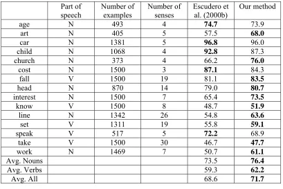
Part of
speech Number of examples Number of senses Escudero et al. (2000b) Our method
age N 493 4 74.7 73.9
art N 405 5 57.5 68.0
car N 1381 5 96.8 96.0
child N 1068 4 92.8 87.3
church N 373 4 66.2 76.0
cost N 1500 3 87.1 84.3
fall V 1500 19 81.1 83.5
head N 870 14 79.0 80.7
interest N 1500 7 65.4 73.5
know V 1500 8 48.7 51.9
line N 1342 26 54.8 63.6
set V 1311 19 55.8 59.1
speak V 517 5 72.2 68.9
take V 1500 30 46.7 47.7
work N 1469 7 50.7 61.1
Avg. Nouns 73.5 76.4
Avg. Verbs 59.3 62.2
Avg. All 68.6 71.7
Table 6. The comparison on 15 frequent works
In another experiment we compared our results with Escudero et al. (2000b) when he separately tested on a group of 15 most frequent words in DSO corpus using an AdaBoost.MH boosting algorithm. Our average result is 71.7% while his is 68.6% (see Table 6 for the detailed comparison).
6.
Discussion
2 http://www.ldc.upenn.edu/
context provides the most informative cues, followed by collocation, and third, by topic context. We can conclude that: by combining three kinds of information, topic context, local context, and collocation, the accuracy of WSD tasks can be improved. This conclusion is confirmed by the results in Table 2 and Table 3, which show that when all three kinds of information are used, instead of using only topic context, the accuracy increases up to about 11.1% for the four words. For DSO corpus, the accuracy increases about 7.3% (see Table 5). These high increases indicate that our approach, which uses more information, can produce better results. The problem here is why there is a difference between the two improvements reported above. We can see that there are more examples in the four words data than in the DSO data. The high data density may be the reason why we achieved a high accuracy, and in this case, the information about part-of-speech may be redundant. That may also be the reason why the accuracy of testing on the four words is higher than its on the DSO corpus.
Among some WSD studies using NB with multiple kinds of information, Leacock and Chodorow (1998) did not use collocation and they only used about 200 examples for training, therefore their result is much lower than ours (less than about 9%). Escudero et al. (2000b) use all kinds of information as in our experiment, but their results were lower than ours by about 3% because they used local context and collocation but with smaller sizes. One more reason why their results are lower than ours may be that both of them used part-of-speech information.
In summary, the most important point here is that WSD using NB with more useful information than usual will give better results.
7.
Conclusion
In this paper, we described our work on a WSD task using a NB classifier with multiple kinds of features. First, we selected the most informative features, and then used a forward sequential selection algorithm to choose the best set of features which include: unordered words in a large context, ordered words in a local context, and collocations. These features do not contain information which needs complicated analysis, such as a syntactic or even a part-of-speech parser. Then, we tested our method on some common words and the large DSO dataset, and obtained results that were better than the best previously published results. Thus, our work shows that WSD using Naive Bayesian classifier with richer features can obtain high accuracies.
In our future research, information about part-of-speech will be checked to determine whether it is useful in the case when we do not have full enough training data. Other important problem which also needs to be considered is how to remove redundant features as a whole, without having to consider the kinds of features.
Acknowledgement
This research is partly conducted as a program for the “Fostering Talent in Emergent Research Fields” in Special Coordination Funds for Promoting Science and Technology by the Japanese Ministry of Education, Culture, Sports, Science and Technology.
References
Bruce, R. and Wiebe, J. 1994. Word-Sense Disambiguation using Decomposable Models. Proceedings of the 32nd Annual Meeting of the Association for Computational Linguistics (ACL), pp. 139-145.
Escudero G., Marquez L., and Rigau G. 2000a. Naive Bayes and Exemplar-Based Approaches to Word Sense Disambiguation Revisited. Proceedings of the 14th European Conference on Artificial Intelligence (ECAI), pp. 421-425.
Escudero G., Màrquez L. and Rigau G. 2000b. Boosting Applied to Word Sense Disambiguation. Proceedings of the 11th European Conference on Machine Learning (ECML), pp. 129-141.
Gale W., Church K., and Yarowsky D. 1992. A Method for Disambiguation Word Sense in a Large Corpus. Computers and Humanities, vol. 26, pp. 415-439.
Leacock, C. and Chodorow, M. and Miller, G. 1998. Using Corpus Statistics and WordNet Relations for Sense Identification. Computational Linguistics, pages 147-165.
Mooney, R. J. 1996. Comparative Experiments on Disambiguating Word Senses: An illustration of the role of bias in machine learning. Proceedings of the Conference on Empirical Methods in Natural Language Processing (EMNLP), pp. 82-91.
Ng, H.T. and Lee, H.B. 1996. Integrating Multiple Knowledge Sources to Disambiguate Word Sense: An Exemplar-Based Approach. Proceedings of the 34th Annual Meeting of the Society for Computational Linguistics (ACL), pp. 40-47.
Pedersen, T. 2000. A Simple Approach to Building Ensembles of Naive Bayesian Classifiers for Word Sense Disambiguation. Proceedings of the North American Chapter of the Association for Computational Linguistics (NAACL), pp. 63-69.