CSEIT1831439 | Received : 16 Feb 2018 | Accepted : 28 Feb 2018 | January-February-2018 [(3) 2 : 131-137]
International Journal of Scientific Research in Computer Science, Engineering and Information Technology © 2018 IJSRCSEIT | Volume 3 | Issue 2 | ISSN : 2456-3307
131
A Survey on Anomalies Detection using Density Based - Rank
Based Outlier Detection Methods
Nehal Patel*, Jayna Shah
Computer Engineering, Sardar Vallabhbhai Patel Institute of Technology, Vasad, Gujarat, India
ABSTRACT
Outlier Analysis is important research area in data mining. Outlier detection is the process of finding an outlying pattern from a given dataset. Outlier detection became an important subject in different knowledge domains. The aim of this paper is to present various Density and Rank based techniques of outlier detection. So a researcher can get direction with these approaches and they can be integrated with any kind of general Applications.
Keywords : Outlier Analysis, Anomaly Detection, Density Based, Rank Based.
I.
INTRODUCTION
Detection of anomalies in data is defined as finding patterns in data that do not confirm to normal behavior or data that do not confirmed to expected behavior, such a data is called as outliers, anomalies, exceptions. Anomaly and Outlier have similar meaning. The analysts have strong interest in outliers because they may represent critical and actionable information in various domains, such as cybersecurity, finance, health, defence, home safety, industry, science and many KDD applications. An Outlier is an observation in data instances, which is different from the others in dataset. There are many reasons due to outliers arise like poor data quality, malfunctioning of equipment. Outlier detection is very much popular in data mining field and it is an active research area due to its various applications like fraud detection, network sensor, email spam, stock market analysis, intrusion detection and also in data cleaning.
II.
RELATED WORKS
Outlier Analysis and Anomaly Detection Approach Layout
An outlier/anomaly is an observation point that is distant from other observations. An anomaly is a “variation from the norm”.
• Density-based: Points that are in relatively low-density regions are considered more anomalous. • Rank-based: A data point is “more anomalous" if it
is not the nearest neighbor of its nearest neighbors.
For each of these approaches, it can be supervised, semi-supervised, or unsupervised.
1) In the supervised case, classification labels are known for a set of “training” data, and all comparisons and distances are with respect to such training data.
2) In the unsupervised case, no such labels are known, so distances and comparisons are with respect to the entire data set.
An unsupervised anomaly detection algorithm should meet the following characteristics:
1. Normal behaviors have to be dynamically defined. No prior training data set or reference data set for normal behavior is needed.
2. Outliers must be detected effectively even if the distribution of data is unknown.
3. The algorithm should be adaptable to different domain characteristics; it should be applicable or modifiable for outlier detection in different domains, without requiring substantial domain knowledge.
a. Density based Approaches
In density based approaches the main idea is to consider the behaviours of a point with respect to its neighbours‟ density values. The neighbourhood is conceptualized by considering k nearest neighbours, where k is either iteratively estimated or is a preassigned integer. The underlying assumption is that if the density at a point p is „smaller‟ than the densities of its neighbours, it must be an anomaly. It examines the k-neighbourhood of a data point, has many good features. For instance, it is independent of the distribution of the data and is capable of detecting isolated objects.
Three well-known density-based algorithms are as following:
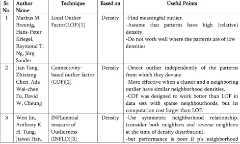
1) LOF [1]
Breunig et al. proposed the following approach to find anomalies in a given dataset. As the name of the algorithm suggests, the Local Outlier Factor (LOF) measures the local deviation of a data point p D with respect to its k nearest neighbors. A point p is declared anomalous if its LOF is „large.‟
The LOF of a point is obtained as described in the following steps:
1. Find the distance, between p and its nearest neighbor. Denote the set of k nearest
neighbors of p by = { { } }.
2. Define the reachability distance of a point q from p, as = max { }.
3. The local reachability density of a point is defined as the inverse of the average reachability distance. Specifically, it is
= ∑ | | .
4. LOF (local outlier factor) of a point p is defined as:
= [∑
| | ]
5. The LOF of each point is calculated, and points are sorted in decreasing order of . If the LOF values are `large', the corresponding points are declared as outliers.
6. To account for k, the final decision is taken as follows: is calculated for selected values of k in a pre-specified range, max is retained, and a p with large LOF is declared an outlier.
2) COF [2]
LOF performs well in many application domains, but its effectiveness will diminish if the density of an outlier is close to densities of its neighbours. To solve such a deficiency of LOF, Tang et al. suggest a new method to calculate the density as described below.
The COF of a point is obtained as described in the following steps:
1. Define the distance between two non-empty sets P and Q as d (P, Q) = min {d (p, q) : p P; q Q}. This can be used to find the minimum distance between a point and a set by treating one of the set as a singleton.
3. The Set-based trail (SBT) is an ordered collection of k-1 edges associated with a given SBN path < p , ,….., > .The edge connects a point o { , ,….., }to and is of minimum distance; i.e., length of is equal to d(o, ) = d({ , ,…..,
}, { ,….. }). Denote the length of edge as l ( ).
4. Given p, the associated SBN path < p , ,….., >, and the SBT < ; , ….., >, the average-chaining distance (A) of p is weighted sum of the lengths of the edges, with larger weights assigned to nearest edges, that is:
= ∑ .
5. Finally, the connectivity-based outlier factor (COF) of a point p is defined as
= [ ]
∑ | |
.
6. As in COF, larger values of denote higher possibility that p is an outlier.
3) INFLO [3]
Jin et al. assigned to each object the degree of being INFLuenced Outlierness (INFLO) and introduce a new idea called „reverse neighbors‟ of a data point when estimating its density distribution.
The INFLO of a point is obtained as described in the following steps:
INFLO the k nearest neighbors and reverse nearest neighbors of an object p are used to obtain a measure of outlierness. Recall that given an object p
1. Reverse Nearest Neighborhood (RNN) of p is defined as
{ } .
Note that has exactly k objects but may not have k objects. In some instances, it may be empty, because for all q , p may not be in any of the set of .
2. The k-influential space for p, denoted as = .
3. The influenced outlierness of a point p is defined as
∑ | |
The common theme among these algorithms is that they all assign outlierness to each object in the data set and an object will be considered as an outlier if its outlierness is greater than a pre-defined threshold (usually the threshold is determined by users or domain experts).
b. Rank Based Approaches
Density based Approaches has the following shortcomings:
• If some neighbors of the point are located in one cluster, and the other neighbors are located in another cluster, and the two clusters have different densities, then comparing the density of the data point with all of its neighbors may lead to a wrong conclusion and the recognition of real outliers may fail.
• The notion of density does not work well for sparse data sets such as a cluster of points on a single straight line. Even if each point in the set has equal distances to its closest neighbors, its density may vary depending on its position in the dataset.
In such situations, to find anomalous observations, the ideal solution is to transform the data so that all regions in the transformed space have similar local distributions. The rank-based approach attempts to achieve this goal.
Here Some Approaches are as following:
1) RBDA [4]
Description of Rank-based Detection Algorithm (RBDA) Algorithm:
1. For p D let q . calculate the rank of p among all neighbors of q; i.e., calculate the set of d (q, o) for all o D – {q} and find the rank of d (q, p) in this set. Let this be .
2. „Outlierness‟ of p, denoted by , is defined as:
= ∑ | | .
If is „large‟ then p is considered an outlier.
3. To determine a criterion for `largeness', let = {p | }where is chosen such that the size of is 75% of the size of D. normalize
as below:
̅
Where,
̅ = | | ∑ and
= | | ∑ ̅ and if the normalized value , then declare that p is an outlier.
2) RADA [5]
Rank-based approach ignores the useful information contained in the distance of the object from other neighbouring objects. To overcome this weakness of RBDA due to “cluster density effect”, adjust the value of RBDA by the average distance of p from its
k−neighbours.
Step by step description of this rank and distance based detection algorithm is given below:
1. Choose three positive integers k, l, .
2. Find the clusters in D by NC(l, ) method.
3. Declare an object O a potential-outlier if it is does not belong to any cluster.
4. Calculate a measure of outlierness:
∑ | |
5. If p is a potential-outlier and ) is large, declare p is an outlier.
3) ODMR [6]
For a point near a dense and large cluster, all of the k nearest neighbors of p may find their neighbors in a close vicinity and p may not be their neighbour; a point near a dense and large cluster may be declared an anomaly, although it may not be so. ODMR modifies the rank of an observation by assigning a weight to overcome the cluster density effect. In ODMR all clusters (including isolated points viewed as a cluster of size 1) are assigned weight 1, i.e., all |C| observations of the cluster C are assigned equal weights = 1/|C|. The “modified-rank” of p with respect to q is defined as the sum of weights associated with all observations within the circle of radius d(q, p) centered at q, and the measure of outlierness is given by Equation (1) with replaced by the modified rank of p.
In this calculate “modified-rank” of p, which is defined as the sum of weights associated with all observations within the circle of radius d (q, p) centered at q; that is modified-rank of p from q = (p) = ∑ { } and sum the “modified-ranks” in q .
Step by step description of the proposed method is as follows:
1. Choose three positive integers k, l, .
2. Find clusters in D by NC(l, ). All objects not belonging to any cluster are declared as potential-outliers.
3. If C is a cluster and p C, then the weight of p is b(p) = 1/|C|.
4. For p D and q , Q denotes the set of points within a circle of radius d (q, p), i.e., Q = {s D | d(q, s) ≤ d(q, p)}. Then the modified-rank of p with respect to q, denoted as (p), is computed as (p) = ∑
[7]. X. Meng and Z. Chen,“On user-oriented measurements of effectiveness of web information retrieval systems,", pp. 527-533, In Proceeding of the international conference on internet computing (2004).
[8]. G. Salton,”Automated text processing: The transformation, analysis, and retrieval of information by computer.”, Addison-Wesley Longman Publishing Co. Inc., Boston (1998). [9]. H. Cao, G. Si, Y. Zhang, and L. Jia, ,”Enhancing
effectiveness of density-based outlier mining scheme with density-similarity-neighbor-based outlier factor", Expert Systems with Applications: An International Journal, vol. 37, December (2010).
[10]. J. Tang, Z. Chen, A. W. Fu, and D. W.