1 Advanced Iterative Procedures for Solving the Implicit Colebrook Equation for Fluid Flow Friction Pavel Praks1,2,*, Dejan Brkić1,*
1European Commission, DG Joint Research Centre (JRC), Directorate C: Energy, Transport and Climate,
Unit C3: Energy Security, Distribution and Markets, Via Enrico Fermi 2749, 21027 Ispra (VA), Italy
2 IT4Innovations National Supercomputing Center, VŠB - Technical University Ostrava, 17. listopadu
2172/15, 708 00 Ostrava, Czech Republic
[email protected] (Pavel Praks) - ORCID id: https://orcid.org/0000-0002-3913-7800 [email protected] (Dejan Brkić) - ORCID id: https://orcid.org/0000-0002-2502-0601
*both authors contributed equally to this study
Abstract: Empirical Colebrook equation from 1939 is still accepted as an informal standard to calculate friction factor during the turbulent flow (4000 < Re < 108) through pipes from smooth with almost
negligible relative roughness (ε/D→0) to the very rough (up to ε/D = 0.05) inner surface. The Colebrook equation contains flow friction factor λ in implicit logarithmic form where it is, aside of itself; λ, a function of the Reynolds number Re and the relative roughness of inner pipe surface ε/D; λ = f (λ, Re, ε/D). To evaluate the error introduced by many available explicit approximations to the Colebrook equation, λ ≈ f(Re, ε/D), it is necessary to determinate value of the friction factor λ from the Colebrook equation as accurate as possible. The most accurate way to achieve that is using some kind of iterative methods. Usually classical approach also known as simple fixed point method requires up to 8 iterations to achieve the high level of accuracy, but does not require derivatives of the Colebrook function as here presented accelerated Householder’s approach (3rd order, 2nd order: Halley’s and Schröder’s method
and 1st order: Newton-Raphson) which needs only 3 to 7 iteration and three-point iterative methods
which needs only 1 to 4 iteration to achieve the same high level of accuracy. Strategies how to find derivatives of the Colebrook function in symbolic form, how to avoid use of the derivatives (Secant method) and how to choose optimal starting point for the iterative procedure are shown. Householder’s approach to the Colebrook’s equations expressed through the Lambert W-function is also analyzed. One approximation to the Colebrook equation based on the analysis from the paper with the error of no more than 0.0617% is shown.
Keywords: Colebrook equation; Colebrook-White; iterative methods; three-point methods; turbulent flow; hydraulic resistances; pipes; explicit approximations; Newton-Rapson; Household’s methods
2 1. Introduction
To evaluate flow resistance in turbulent flow through pipes, from smooth to rough, the empirical Colebrook equation is in common use (1) {Colebrook 1939}:
√ = −2 ∙ log
.
∙√ + . ∙ (1)
In the Colebrook equation λ represents Darcy flow friction factor, Re Reynolds number and ε/D relative roughness of inner pipe surfaces (all three quantities are dimensionless).
The experiment performed by Colebrook and White {Colebrook and White 1937} dealt with flow of air through one pipe (diameter D=53.5mm and length L=6m) with six different roughness of inner surface of the pipe artificially simulated with various mixtures of two sizes of sand grain (0.035mm and 0.35mm diameter) to simulate conditions of inner pipe surface from almost smooth to very rough. The sand grains were fixed using a sort of bituminous adhesive waterproof insulating compound to form five types of relatively uniform roughness of inner pipe surfaces while the sixth one was without sand, i.e. it was left smooth. The experiment revealed, contrary to the previous, that flow friction, λ does not have a sharp transition from the smooth to the fully rough law of turbulence. This evidence Colebrook {Colebrook 1939} later captured in the today famous and widely used empirical equation; Eq. (1). The Colebrook function relates the unknown flow friction factor λ as function of itself, the Reynolds number Re and the relative roughness of inner pipe surface ε/D; λ=f(λ, Re, ε/D). It is valid for 4000<Re<108 and for 0<ε/D<0.05. The Colebrook equation is transcendent and thus cannot be solved in
terms of elementary functions {Sonnad and Goudar 2007, Brkić 2011a, Mikata and Walczak 2016, Vatankhah 2018}. Although empirical, and therefore with questionable accuracy its precise solution is sometimes essential in order to repeat or to evaluate previous findings in a concise way {Schockling et al. 2007, Allen et al. 2007, Langelandsvik et al. 2008, Clamond 2009}.
Few approaches are available today for solving Colebrook equation:
(1) Graphical solution – Moody diagram: To represent the Colebrook equation graphically, Rouse in 1942 had developed appropriate diagram which Moody later adopted in 1944 in famous diagram widely used in the past in engineering practice {Moody 1944, LaViolette 2017}. The diagram was preferred because the Colebrook equation is implicitly given. Today, graphical solution has only value for educational purposes.
(2) Iterative solution of the Colebrook equation:
(2.a.) Simple fixed point iterative method. The simple fixed point iterative method {Brkić 2017a} is in common use for solving accurately the Colebrook equation (special case of the Colebrook equation for Re→∞ gives explicit form valid only for the fully turbulent flow in rough pipes {Schultz and Flack 2007, Herwig et al. 2008, Brkić 2012a, Brkić 2016a} but which can be used as initial starting point for all cases covered by the Colebrook equation λ0=f(ε/D)→Eq. (2); now
3 the procedure λi+1=f(λi; Re; ε/D); i=i+1 goes until λi≈λi+1, where we set λi+1-λi≤10-8). It usually
reaches the satisfied accuracy after about 8 iterations.
(2.b.) Householder’s iterative methods. On the other hand, Newton’s method (also known as the Newton-Raphson method {Cajori 1911, Ypma 1995, Abbasbandy 2003}) needs only 3 to 7 iterations to reach the same level of accuracy. A shortcoming of Newton’s method is that it additionally requires the first derivative of the Colebrook’s function (here we show analytical form of the first derivative including the symbolic form generated in MATLAB {Shampine 2007}). Also knowing that the Newton-Raphson method is 1st order of Householder’s method
{Householder 1970, Griffiths and Smith 2006}, we analyze 2nd order which is known as Halley’s
{Halley 1694} and Schröder’s {Schröder 1870, Petković et al. 2010} method, and also 3rd order.
The 3rd order methods use the third, the second and the first derivative, 2nd order the second
and the first while 1st order use only the first derivative. Today, all mentioned types of iterative
solutions can easily be implemented in software codes and they has been accepted as the most accurate way for solving the Colebrook equation and hence they are preferred compared to the graphical solution.
(2.c.) Three-point iterative methods. Three-point iterative methods needs only 1 iteration in three points x0, y0 and z0 (three internal iterations) to achieve high level of accuracy {Džunić et
al. 2011, Petković et al. 2014, Sharma and Arora 2016,}. x0 is initial starting point, y0 is auxiliary
step, while z0 is the solution. Three-point methods are very accurate and can reach high
accuracy some cases even after 1 to 2 iterations. Also slightly less accurate two-point methods exist.
(3) Approximations of the Colebrook equation: Colebrook’s equation can be expressed in explicit form only in an approximate way; λ≈f(Re, ε/D) {Gregory and Fogarasi 1985, Zigrang and Sylvester 1985, Giustolisi et al. 2011, Genić et al. 2011, Brkić 2011b, Brkić 2012b, Winning and Coole 2013, Brkić and Ćojbašić 2017}. Numerous explicit approximations to the Colebrook equation are available in literature {Gregory and Fogarasi 1985, Zigrang and Sylvester 1985, Brkić 2011b, Genić et al. 2011, Brkić 2012b, Winning and Coole 2013, Brkić and Ćojbašić 2017}. Iterative solution as the most accurate method is used for evaluation of accuracy of such approximations. Also, based on our findings, we provide an approximation; Eq. (28) with the error of no more than 0.69% and 0.0617%. The Colebrook equation also can be approximately simulated using Artificial Neural Networks {Özger and Yıldırım 2009, Brkić and Ćojbašić 2016, Bardestani et al. 2017}.
(4) Lambert W-function: Until now only one known way to express the Colebrook equation exactly in explicit way is through the Lambert W-function; λ=W(Re, ε/D) {Keady 1998, Clamond 2009, Brkić 2011a, Brkić 2012c}, where further evaluation of the Lambert W-function can be only approximate {Corless et al. 1996, Boyd 1998, Barry et al. 2000, Hayes 2005, Mező and Baricz 2017}. Here we show procedure how to solve the Lambert W-function using Householder’s iterative procedure (2nd order: Halley’s method and 1st order: Newton-Raphson). Also approach
4 In this paper, we show Householder’s iterative procedures (3rd order, 2nd order: Halley’s {Scavo and Thoo
1995} and Schröder’s method and 1st order: Newton-Raphson) and one example of the three-point
methods with additional recommendations in order to solve the empirical Colebrook equation which is implicitly given in respect to flow friction factor λ. The goal of this paper is to show improved iterative solutions that can obtain value of the unknown friction factor λ accurately after the least possible number of iterations. Additionally we developed a strategy how to choose the best starting point {Kornerup and Muller 2006} for the iterative procedure in the domain of interest of the Colebrook equation, how to generate required symbolic derivatives to the Colebrook equation in MATLAB and how to avoid use of derivatives (Secant method). Finally, we use findings from our paper to present a novel explicit approximation of the Colebrook equation, which would be interesting for engineering practice. We also present distribution of the relative error in respect of the presented approximation over the applicability domain of the Colebrook equation.
To evaluate efficiency of the presented methods unknown flow friction factor λ is calculated for two pairs of the Reynolds number Re and relative roughness of inner pipe surfaces ε/D; 1) {Re=5·106,
ε/D=2.5·10-5}→λ=0.010279663295529, and 2) {Re=3·104, ε/D=9·10-3}→λ=0.038630738574792.
2. Initial estimate of starting point for the iterative procedures
The starting point is a significant factor in convergence speed in three-point and Householder’s method {Kornerup and Muller 2006} and there are different methods to choose a good start but here we examine 1) Starting point as function of input parameters, and 2) Initial starting point with the fixed value.
One of the essential issues in every iterative procedure is to choose good starting point {Moursund 1967, Taylor 1970}. Here we try to find the fixed starting point (initial value of the flow friction factor λ0
or the related transmission factor = ) valid for all cases from the practical domains of applicability of the Colebrook equation which is; Reynolds number Re; 4000<Re<108 and the relative roughness ε/D;
5 further can be evaluated only approximately through Householder’s iterative procedures which also require the appropriate initial starting point. The analysis of this initial starting point has wider applicability, because the Lambert W-function has extensive use in many branches of physics and technology {Valluri et al. 2000, Hosseini et al. 2014}.
2.1. Starting point as function of input parameters
2.1.1. Star ng point as func on of the rela ve roughness ε/D (when Re→∞)
Special case of the Colebrook equation when Re→∞ physically means that the flow friction factor λ in that case depends only on ε/D; for Re→∞, λ=f(ε/D), i.e. the flow friction factor λ is not implicitly given {Brkić 2016a}. In that way starting point can be calculated using explicit equation which has only one variable; λ0=f(ε/D); Eq. (2). The results obtained in that way are accurate only for the case Re→∞ but for
the smaller values of Re which corresponds to the smooth turbulent flow the error can goes up to 80% {Brkić 2011c, Brkić 2012a}. Anyway, in that way calculated value can be efficiently used as initial starting guess for iterative procedure for the whole domain of applicability of the Colebrook equation.
= = −2 ∙ log . ∙ (2)
The initial starting point obtained using the previous equation is referred as “traditional”, it introduces the maximal relative error of 80% over the domain of applicability of the Colebrook equation where the error can be neglected in case of fully developed turbulent flow through the pipes with very rough inner surface. To reach accuracy of λi+1-λi≤10-8 usually 6 steps are enough regarding the Newton-Raphson
method (Figure 1).
Figure 1. “Slow area” which requires 6 iterations to reach accuracy of 10-8 regarding the “traditional”
6 2.1.2 Starting point obtained using approximations to the Colebrook equation
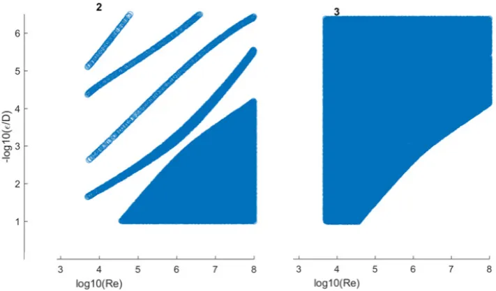
Every approximation to the Colebrook equation; λ≈f(Re, ε/D) can be used to put initial starting point as close as possible near the final accurate solution {Brkić 2011b}. For example, using one of the approximation with the error of up to 10% for calculation of initial starting point =√ , the final accurate value of the flow friction factor λ is reached in the worst case scenario after 3 iterations using Colebrook’s equation and one of the procedures from Section 3.2. After 3 iterations, the whole practical domain of applicability of the Colebrook equation is covered with the difference between the two final iterations less than 10-8; λ
i+1-λi≤10-8 (Figure 2). In average, the method requires 2.7 iterations in average
for all cases with set precision (stopping criterion) very close to zero (about 10-8) when calculation goes
through the transmission factor x. The results from Figure 1 are from the 65536 pairs of the Reynolds number Re and the relative roughness ε/D over the domain of applicability of the Colebrook equation domain (values of the Reynolds number Re between 4000 and 108 and the relative roughness ε/D
between 0 and 0.05, dividing them into 256 points each).
Figure 2. Area in which 2 iterations (left), and 3 iterations (right) are sufficient to calculate the flow friction factor λ with accuracy of 10-8 using Colebrook equation solved in Newton’s procedure when
calculation goes through the transmission factor x and using approximation with error of up to 10%
2.2 Fixed initial starting point
7 2.2.1 Fixed initial starting point for the Newton-Raphson method
The “center of gravity” for the “slow area” in which the Newton-Raphson method requires increased number of iterations is shown in Figure 1. The “center of gravity” has coordinates: log(Re)=4.4322→Re≈27000 and –log(ε/D)=5.7311→ε/D≈1.85·10-6 for which the flow friction factor λ and
the corresponding transmission factor =
√ can be calculated using any of the available methods. In
that way calculated x, became the starting point x0 for all combinations of the Reynolds number Re and
the relative roughness ε/D in the domain of applicability of the Colebrook equation. With this new starting point x0 the maximal required number of iterations is 4 (Figure 3), while before in the worst case
was 6 (Figure 1) when the starting point x0 was obtained through the “traditional formula” for this
purpose; Eq. (2), all valid for the case when the flow friction factor λ is calculated with accuracy of λi+1
-λi≤10-8 using Colebrook equation solved in Newton’s procedure when calculation goes through the
transmission factor x.
The physical interpretation of this “slow area” is in the fact that this area corresponds to the initial zone of turbulent flow through smooth pipes while Eq. (2) is accurate only for the fully developed turbulent flow through rough pipes. So, Eq. (2) can already obtain accurate solution in the case of fully developed turbulent flow through rough pipes even without the iterative process, where Eq. (2) introduces the relative error of almost 80% in the case of initial phases of turbulent flow through smooth pipes.
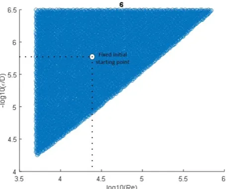
With the initial starting point fixed at the “centre of gravity” of the “slow area”, in the worst cases, maximum 4 iterations as shown in Figure 3 are enough for the required accuracy of 10-8 (before with the
“traditional” version of initial value provided using Eq. (2) was 6 as indicated in Figure 1). The new fixed starting point is set as λ0=0.024069128765100981, i.e. x0=6.44569593948452. It corresponds to
log(Re)=4.4322→Re≈27000 and –log(ε/D)=5.7311→ε/D≈1.85·10-6.
Figure 3. Decreased maximal number of required iterations from 6 to 4 to reach accuracy of 10-8 for
solving Colebrook’s equation in Newton’s procedure when calculation goes through the transmission factor x where the initial starting point is with the fixed value: x0=6.44569593948452
0 1 2 3 4 5 6 7 8
log10(Re)
0 1 2 3 4 5 6
8 The new starting point x0=6.44569593948452 is very robust and it seems to be an optimal starting point
for all combinations when calculation goes through the transmission factor =
√ as explained in
Section 3.2.
2.2.2 Fixed initial starting point for the Halley and Schröder method
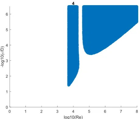
Starting point for calculation through the Halley and Schröder method using Eq. (2) requires in the worst cases up to 4 iterations to reach the required accuracy (Figure 4). Compared with the Newton-Raphson method it is improvement of two iterations; up to 6 iterations required in Figure 1 and up to 4 iterations in Figure 4. The “worst-case” area for Halley and Schröder’s method that requires 4 iterations using staring point Eq. (2) has coordinates: {log10(Re)=5.3108→Re≈204550; –log10(ε/D)=4.9431→ε/D≈1.14·10 -5}→ λ
0=0.015663210285978339; i.e. x0=7.990256504. This value is the new optimal initial starting point
in the case of the Halley and Schröder method.
Figure 4. “Slow area” which requires 4 iterations to reach accuracy of 10-8 regarding the “traditional”
option for the starting point calculated through Eq. (2), for solving Colebrook’s equation in Halley’s and Schröder’s procedure when calculation goes through the transmission factor x
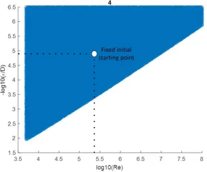
With the new initial starting point x0=7.990256504, three iterations are required at maximum to reach
9 Figure 5. Decreased maximal number of required iterations from 4 to 3 to reach accuracy of 10-8 for
solving Colebrook’s equation in Halley’s and Schröder’s procedure when calculation goes through the transmission factor x where the initial starting point is with the fixed value: x0=7.990256504
2.2.3 Fixed initial starting point for the three-point iterative methods
Optimal normalized parameters for the fixed initial starting point for the three-point iterative methods explained in Section 3.4. of this paper {Džunić et al. 2011, Petković et al. 2014, Sharma and Arora 2016} are: {log10(Re)=4.90060379974617→Re=79543.33576; –log(ε/D)=5.33355157079189→ε/D=4.63926·10
-6}→λ0=0.018904186734624→x
0=7.273124147. The Džunić–Petković method is shown in Section 3.4.
Additional recommendations about initial starting point regarding the three-point iterative methods can be found in {Yun 2008}.
2.3 Starting point for the Lambert W-expressed Colebrook equation
The friction factor λ in the Colebrook equation can be expressed in explicit way through the Lambert W-function { Keady 1998, Sonnad and Goudar 2006, Sonnad and Goudar 2007, Clamond 2009, Brkić 2011a, Brkić 2012b, Brkić 2017b}. The Lambert W-function further can be evaluated using some types of Householders iterative methods as shown in Section 3.5 of this paper.
The Colebrook equation in a closed form through the Lambert W-function can be expressed in two ways; Eqs. (3) and (4). The first expression is, Eq. (3) {Goudar and Sonnad 2003, Brkić 2011a, Brkić 2012b, Brkić 2017b}:
√ = −2 ∙ log
∙ . ∙ ( )
∙ ( ) + . ∙ = −2 ∙ log 10
( )
( )+
. ∙ (3)
where = ∙ ( )
10 The argument of the Lambert W-function in this case depends only on the Reynolds number; λ0=Re/2.18. Knowing that the practical range of the Reynolds number goes from 4000 to 108, the
argument of the Lambert W-function is goes from about 1835 to 45871560, where W(1835)=5.763291081 and W(45871560)=14.93748223. The Halley procedure is fast and any initial starting point can be chosen between 5 and 15, but the Newton-Raphson method is very slow and we found that for the best results the initial starting point 15 has to be chosen. Note that for W(45871560)=14.93748223, the Newton-Raphson procedure does not work in Excel for the values of initial starting point lower than 8.814.
Due to transformations of coefficients, Eq. (3) can introduce the relative error up to 2% and should be considered as explicit approximation to the Colebrook equation rather to its equivalent {Brkić 2011d}. The second expression is; Eq. (4): {Keady 1998, Sonnad and Goudar 2004}:
= ( )∙ ( ) − ∙
. ∙ . (4)
Where = ∙ . ∙ .∙ ∙ ( )− ln ∙ ( )∙ .
Argument of the Lambert W-function in this case is eα which for certain combinations of Re and ε/D
from the practical domain of the Colebrook equation is too big to be calculated in registers of computers {Sonad and Goudar 2004, Brkić 2012c, Vatankhah 2018}. This can be overwhelmed with the Wright Omega function; ( ) = ( ) {Wright 1959a, Wright 1959b, Corless and Jeffrey 2002, Rollmann and Spindler 2015, Biberg 2017}.
The argument of the Lambert W-function in this case, exp(α0) depends on both Re and ε/D, but as
explained due to exponential form the calculation is not always possible and because of that limited possibility of use the appropriate starting point in this case is not evaluated {Goldberg 1991, Sonnad and Goudar 2004, Kornerup and Matula 2010, Brkić 2012c}.
3. Iterative Methods Adopted for the Colebrook Equation
Householder's method {Householder 1970} is a numerical algorithm for solving the nonlinear equation such as Colebrook’s. During the Householder’s procedure, in successive calculation, i.e. in iterative cycles the original assumed value of the unknown quantity (initial starting point {Kornerup and Muller 2006}) needs to be brought as much as possible close to the real value of the quantity using the least possible number of iterations. The same situation is with the three-point methods {Sharma and Arora 2016}.
The following types of the method are used in this paper: 1st order Householder’s method
(Newton-Raphson {Cajori 1911, Ypma 1995}), 2nd order (Halley {Gander 1985, Gutierrez and Hernández 2001} and
11 these methods require calculation of the derivatives which is usually underlined as the most important shortcoming of Householder’s and three-point methods compared with the simple fixed point procedure in respect of the Colebrook equation. The Newton-Raphson and three-point method require only the first derivative, the Halley and Schröder the first and the second derivative, while the 3rd
requires the first, the second and the third derivative. In addition to the first derivate in analytical form, all required derivatives of the Colebrook function we present also in a simple and computationally inexpensive symbolic form. The derivatives in symbolic form were generated in MATLAB. In addition, the Secant method which does not require derivatives is shown as a variant of the Newton-Raphson method {Varona 2002}.
All shown approaches with Householder’s methods in our case usually require only 2 to 4 iterations to reach final accurate solution {Yamamoto 2001}. This number can be slightly higher depending on the chosen method where Secant method requires by default 1-2 iterations more. Also some simple transformations of the Colebrook equation, such as introduction of the transmission factor in form of the shift =
√ ; can reduce number of required iterations. Knowing that the right form of equation is
essential for all types of Householder’s methods, here are examined two at first look very similar options: 1) direct calculation of λ in Section 3.1, and 2) indirect calculation of λ through transmission factor =
√ in Section 3.2.
Finally, the Colebrook equation can be rewritten in explicit form through the Lambert W-function {Keady 1998, Sonnad and Goudar 2004, Brkić 2012c, Brkić 2012d} and the Lambert W-function is solved in Section 3.5 using the Newton-Raphson and the Halley procedure.
3.1. Direct calculation of λ with derivative calculated in analytical way
The proposed technique requires the Colebrook equation in the form f(λ, Re, ε/D)=0; Eq. (5) where λ is treated as variable, the first derivative f’(λ, Re, ε/D); Eq. (6) of the Colebrook equation with respect of λ and the initial value of the friction factor λ0 as starting point. Most probably, the function will have
residue f/f’≠0 which needs to be minimized through the iterative process. Here are the required steps for the Newton-Raphson procedure:
-The Colebrook equation in the form f(λ, Re, ε/D)=0; (5):
( ) =
| |+ 2 ∙ log
.
∙ | |+ . ∙ = 0
: ( )
(5)
-The first derivative f’ with respect of λ in exact analytical way (6):
( ) = ( ) = − ∙
| | ∙ 1 +
∙ .
( )∙ ∙ .
∙ | | . ∙
( )
12 -Initial value λ0 selected as explained in Section 2 of this paper in order to calculate the residue f/f’ and
start the iterative procedure; Eq. (7):
= − ( )( ) = − | | ∙
. ∙ | | . ∙
∙
| | ∙
.
∙ .
∙ | | . ∙
(7)
The procedure λi+1=λi-f(λi)/f’(λi) needs to be followed until the residue f(λi)/f’(λi)≈0.
The explained Newton-Raphson procedure is shown in Tables 1 and 2 for two numerical examples: 1) {Re=5·106, ε/D=2.5·10-5}→ λ=0.010279663295529, and 2) {Re=3·104, ε/D=9·10 -3}→λ=0.038630738574792. As explained in Section 2 of this paper, the initial starting point λ
0 in Table 1
depends on input parameters, while in Table 2 it is with the fixed value.
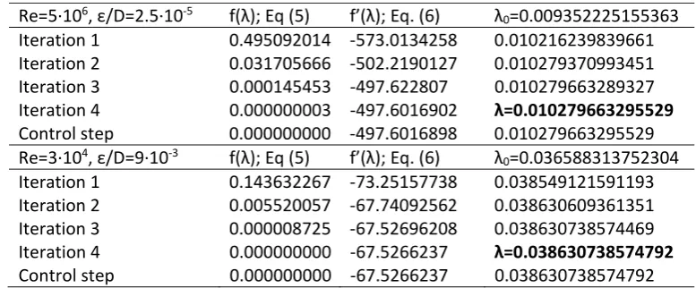
Table 1. Newton-Raphson procedure; Option 1: Starting point λ0 depends on input parameters – Eq. (2),
calculation of λ – Eq. (7), analytical derivative f’(λ) – Eq. (6)
Re=5·106, ε/D=2.5·10-5 f(λ); Eq (5) f’(λ); Eq. (6) λ
0=0.009352225155363
Iteration 1 0.495092014 -573.0134258 0.010216239839661 Iteration 2 0.031705666 -502.2190127 0.010279370993451 Iteration 3 0.000145453 -497.622807 0.010279663289327 Iteration 4 0.000000003 -497.6016902 λ=0.010279663295529 Control step 0.000000000 -497.6016898 0.010279663295529 Re=3·104, ε/D=9·10-3 f(λ); Eq (5) f’(λ); Eq. (6) λ
0=0.036588313752304
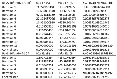
13 Table 2. Newton-Raphson procedure; Option 2: Fixed initial starting point λ0=0.024069128765100981
from Section 2.2.1, calculation of λ – Eq. (7), analytical derivative f’(λ) – Eq. (6) Re=5·106, ε/D=2.5·10-5 f(λ); Eq (5) f’(λ); Eq. (6) λ
0=0.024069128765101
Iteration 1 -3.554956084 -139.7424853 -0.001370207567104 Iteration 2 17.630891548 -10069.59089 0.000380696888310 Iteration 3 42.275315189 -68216.8306 0.001000416608714 Iteration 4 22.325487096 -16105.99979 0.002386576262278 Iteration 5 10.932300910 -4398.30144 0.004872149626988 Iteration 6 4.615550920 -1516.202309 0.007916302041016 Iteration 7 1.426053458 -734.846953 0.009856914916156 Iteration 8 0.217044469 -529.7853757 0.010266598684182 Iteration 9 0.006507144 -498.5470019 0.010279650902858 Iteration 10 0.000006167 -497.602585 0.010279663295518 Iteration 11 0.000000000 -497.6016898 λ=0.010279663295529 Control step 0.000000000 -497.6016898 0.010279663295529 Re=3·104, ε/D=9·10-3 f(λ); Eq (5) f’(λ); Eq. (6) λ
0=0.024069128765101
Iteration 1 1.391712394 -137.1740994 0.034214720386916 Iteration 2 0.326434508 -80.9945153 0.038245048943635 Iteration 3 0.026240732 -68.54940037 0.038627849256271 Iteration 4 0.000195117 -67.53419088 0.038630738412914 Iteration 5 0.000000011 -67.52662412 λ=0.038630738574792 Control step 0.000000000 -67.5266237 0.038630738574792
Here shown direct calculation of the unknown flow friction factor λ is sensitive on the chosen initial starting point λ0 {Kornerup and Muller 2006}. The fixed initial point λ0 chosen as in Section 2.2 for in
some cases requires increased number of iterations to reach the final solution although the procedure still maintains very good convergent properties {Yamamoto 2001, Varona 2002}. To reduce number of required iterations, use of some of the explicit approximation to the Colebrook equation are advised in order to bring the initial starting point λ0 as close as possible near the final calculated value. Therefore,
the approach with the fixed starting point as explained in Section 2.2 of this paper for all domain of the Colebrook equation, in this case cannot be advised in comparison to the approach with the starting point obtained using approximations as explained in Section 2.1.
14 3.2. Indirect calculation of λ through the transmission factor =
√
The appropriate form of the function is essential to reduce number of required iteration to reach the final solution. In order to accelerate the procedure an appropriate shift =
√ is used to provide some
kind of linearization of the problem.
The Newton-Raphson procedure with these changes has similar steps as already shown:
-Shift in form of the transmission factor =√ should be introduced in order to transform the Colebrook equation in form f(x, Re, ε/D)=0; Eq. (8):
( ) = + 2 ∙ log . ∙ + . ∙ = 0
: ( )
(8)
The first derivative of Eq. (8) in respect to the transmission factor x can be calculated analytically, but also in symbolic form (where both approaches give identical results); Sections 3.2.1 and 3.2.2.
3.2.1 Indirect calculation of λ through the transmission factor =
√ with the derivative calculated
analytically
-The first derivative f’ with respect of x can be obtained analytically; Eq. (9), (also Eq. (11) gives the same results):
′( ) = ( ) = 1 + 2 ∙
. ∙ ( )
. ∙ .
∙ ( )
(9)
-Initial value of the flow friction factor λ0 should be chosen and the residue f/f’ calculated in order to
start the Newton-Raphson procedure; Eq. (10):
= − ( )( ) = − ∙
. ∙ . ∙
∙
. ∙ ( ) . ∙ . ∙
(10)
The procedure xi+1=xi-f(xi)/f’(xi) should be followed until the residue f(xi)/f’(xi)≈0. Then the final solution
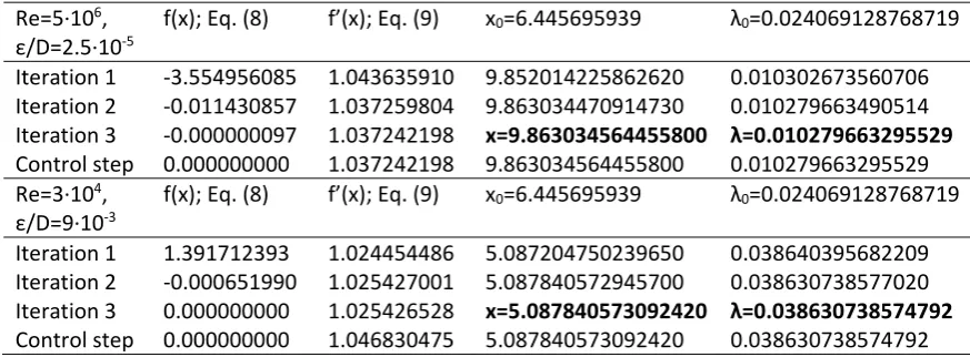
15 Table 3. Newton-Raphson procedure; Option 3: fixed initial starting point
x0=6.445695939→λ0=0.024069128765101 from Section 2.2.1, indirect calculation of λ through the
transmission factor x – Eq. (10), analytical derivative f’(x) – Eq. (9) Re=5·106,
ε/D=2.5·10-5
f(x); Eq. (8) f’(x); Eq. (9) x0=6.445695939 λ0=0.024069128768719
Iteration 1 -3.554956085 1.043635910 9.852014225862620 0.010302673560706 Iteration 2 -0.011430857 1.037259804 9.863034470914730 0.010279663490514 Iteration 3 -0.000000097 1.037242198 x=9.863034564455800 λ=0.010279663295529 Control step 0.000000000 1.037242198 9.863034564455800 0.010279663295529 Re=3·104,
ε/D=9·10-3
f(x); Eq. (8) f’(x); Eq. (9) x0=6.445695939 λ0=0.024069128768719
Iteration 1 1.391712393 1.024454486 5.087204750239650 0.038640395682209 Iteration 2 -0.000651990 1.025427001 5.087840572945700 0.038630738577020 Iteration 3 0.000000000 1.025426528 x=5.087840573092420 λ=0.038630738574792 Control step 0.000000000 1.046830475 5.087840573092420 0.038630738574792
Approach with the indirect calculation of λ through the transmission factor x is much more stable compared with the direct calculation of λ as can be seen from Tables 2 and 3 comparing the number of required iterations to reach the same accuracy (11 iterations for the direct approach compared with only 3 iterations in the indirect approach using fixed starting point x0=6.445695939 for Re=5·106,
ε/D=2.5·10-5).
3.2.2 Indirect calculation of λ through the transmission factor =√ with the symbolic derivative
-The exact analytical expression of the first derivative f’ with respect of x can be obtained in MATLAB; Eq. (11), results are the same as using Eq. (9):
′( ) = ( ) = .
∙ ( )∙ ∙ ∙∙ + 1 =
∙ ( )∙ ∙ ( )∙ ∙
( )∙ ∙ ∙ ∙
( )
(11)
-Initial value of the flow friction factor λ0 should be chosen and the residue f/f’ calculated in order to
start the Newton-Raphson procedure; Eq. (12):
= − ( )( ) = − ∙
. ∙ . ∙
. ∙ . ∙ ∙
. ∙ . ∙ ∙
(12)
The procedure xi+1=xi-f(xi)/f’(xi) should be followed until the residue f(xi)/f’(xi)≈0. Then the final solution
16 The iterative procedure can be accelerated using Halley’s formula instead of the Newton-Raphson; Eq. (13):
= −
( ) ( ) ( )· ( )
∙ ( )
= − ∙ ( )∙ ( )
∙ ( ) ( )∙ ( ) (13)
In general x1=xi+1 and x0=xi; i=0 to n, where n+1 is the final iteration in which xn≈xn+1.
The second derivative f’’(x) in respect of x is required; Eq. (14):
′′( ) = ′( ) = .
∙ ( )∙ ∙ ∙∙ = ( )∙ ∙ ∙ ∙
( )
(14)
The Newton-Raphson method belongs to the 1st order, and the Halley to the 2nd order of Householder’s
method while the 3rd order can be expressed using Eq. (15):
= − ∙ ( )∙ ( ) ∙ ( ) ∙ ( )
∙ ( ) ∙ ( )∙ ( )∙ ( ) ( ) ∙ ( ) (15)
Again, x1=xi+1 and x0=xi; i=0 to n, where n+1 is final iteration in which xn≈xn+1.
The required 3rd derivative f’’’(x) can be expressed using Eq. (16):
( ) = ( ) = .
∙ ( )∙ ∙ ∙∙ = ( )∙ ∙ ∙ ∙
( )
(16)
Also here one has to be underlined that the Halley method {Brown 1977} is not the unique Householder’s method of the 2nd order {Householder 1970}. For example Schröder's method {Schröder
1870} belongs also to the group; Eq. (17):
= − ( )( )− ( )∙ ( )
∙ ( )
ö
(17)
Further x1=xi+1 and x0=xi; i=0 to n, where n+1 is final iteration in which xn≈xn+1.
Using the presented Householder procedures; 1st order: the Newton-Raphson, 2nd: Halley, and 3rd, the
unknown flow friction factor λ should be calculated for the two given pairs of the Reynolds number Re and the relative roughness ε/D: 1) {Re=5·106, ε/D=2.5·10-5}→ λ=0.010279663295529, and 2) {Re=3·104,
ε/D=9·10-3}→λ=0.038630738574792. The calculation presented in Tables 4-7 is through the transmission
17 transmission factor x – Eq. (12), the symbolic derivative f’(x) – Eq. (11)
Re=5·106,
ε/D=2.5·10-5
f(x); Eq. (8) f’(x); Eq. (11) x0=10.34052343 λ0=0.009352225155363
Iteration 1 0.495092014 1.036495031 9.862863625818000 0.010280019623455
Iteration 2 -0.000177305 1.037242471 9.863034564433310 0.010279663295576
Iteration 3 0.000000000 1.037242198 x=9.863034564455800 λ=0.010279663295529
Control step 0.000000000 1.037242198 9.863034564455800 0.010279663295529
Re=3·104,
ε/D=9·10-3
f(x); Eq. (8) f’(x); Eq. (11) x0=5.227918429 λ0=0.036588313752304
Iteration 1 0.143632267 1.025322691 5.087833489750430 0.038630846139210
Iteration 2 -0.000007263 1.025426533 5.087840573092400 0.038630738574793
Iteration 3 0.000000000 1.025426528 x=5.087840573092420 λ=0.038630738574792
Control step 0.000000000 1.025426528 5.087840573092420 0.038630738574792
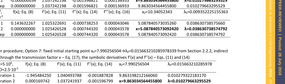
Table 5. Halley procedure; Option 5: fixed initial starting point x0=7.990256504→λ0=0.015663210285978339 from Section 2.2.2, indirect
calculation of λ through the transmission factor x – Eq. (13), the symbolic derivatives f’(x) and f’’(x) – Eqs. (11) and (14) Re=5·106,
ε/D=2.5·10-5
f(x); Eq. (8) f’(x); Eq. (11) f’’(x); Eq. (14) x0=7.990256504 λ0=0.015663210285978
Iteration 1 -1.945484250 1.040493788 -0.001887828 9.863203600915390 0.010279310950983
Iteration 2 0.000175332 1.037241928 -0.001596798 x=9.863034564455800 λ=0.010279663295529
Control step 0.000000000 1.037242198 -0.001596821 9.863034564455800 0.010279663295529
Re=3·104,
ε/D=9·10-3
f(x); Eq. (8) f’(x); Eq. (11) f’’(x); Eq. (14) x0=7.990256504 λ0=0.015663210285978
Iteration 1 2.973246188 1.023435376 -0.000632309 5.087698791122220 0.038632891696967
Iteration 2 -0.000145387 1.025426633 -0.000744326 x=5.087840573092420 λ=0.038630738574792
Control step 0.000000000 1.025426528 -0.000744320 5.087840573092420 0.038630738574792
doi:10.20944/preprints201807.0505.v1
Advances in Civil Engineering
2018
,
2018
, 5451034;
18
Table 6. 3rd order Householder’s procedure; Option 6: starting point x
0 depends on input parameters – Eq. (2), indirect calculation of λ through
the transmission factor x – Eq. (15), the symbolic derivatives f’(x), f’’(x) and f’’’(x) – Eqs. (11), (14) and (16) Re=5·106,
ε/D=2.5·10-5
f(x); Eq. (8) f’(x); Eq. (11) f’’(x); Eq. (14) f’’’(x); Eq. (16) x0=10.34052343 λ0=0.009352225155363
Iteration 1 0.495092014 1.036495031 -0.001533392 0.000128855 9.863034531578420 0.010279663364062
Iteration 2 -0.000000034 1.037242198 -0.001596821 0.000136933 x=9.863034564455800 λ=0.010279663295529
Control step 0.000000000 1.037242198 -0.001596821 0.000136933 9.863034564455800 0.010279663295529
Re=3·104,
ε/D=9·10-3
f(x); Eq. (8) f’(x); Eq. (11) f’’(x); Eq. (14) f’’’(x); Eq. (16) x0=10.34052343 λ0=0.009352225155363
Iteration 1 0.143632267 1.025322691 -0.000738253 0.000043046 5.087840573035260 0.038630738575660
Iteration 2 0.000000000 1.025426528 -0.000744320 0.000043578 x=5.087840573092420 λ=0.038630738574792
Control step 0.000000000 1.025426528 -0.000744320 0.000043578 5.087840573092420 0.038630738574792
Table 7. Schröder procedure; Option 7: fixed initial starting point x0=7.990256504→λ0=0.015663210285978339 from Section 2.2.2, indirect
calculation of λ through the transmission factor x – Eq. (17), the symbolic derivatives f’(x) and f’’(x) – Eqs. (11) and (14) Re=5·106,
ε/D=2.5·10-5
f(x); Eq. (8) f’(x); Eq. (11) f’’(x); Eq. (14) x0=7.990256504 λ0=0.015663210285978
Iteration 1 -1.945484250 1.040493788 -0.001887828 9.863198212166060 0.010279322183170
Iteration 2 0.000169742 1.037241937 -0.001596799 x=9.863034564455800 λ=0.010279663295529
Control step 0.000000000 1.037242198 -0.001596821 9.863034564455800 0.010279663295529
Re=3·104,
ε/D=9·10-3
f(x); Eq. (8) f’(x); Eq. (11) f’’(x); Eq. (14) x0=7.990256504 λ0=0.015663210285978
Iteration 1 2.973246188 1.023435376 -0.000632309 5.087701128882780 0.038632856193927
Iteration 2 -0.000142990 1.025426632 -0.000744326 x=5.087840573092420 λ=0.038630738574792
Control step 0.000000000 1.025426528 -0.000744320 5.087840573092420 0.038630738574792
doi:10.20944/preprints201807.0505.v1
Advances in Civil Engineering
2018
,
2018
, 5451034;
19 3.3. Secant method
Secant method is similar to the Newton-Raphson, it requires two starting points λ0 and λ-1 but doesn’t
require calculation of the derivatives {Varona 2002}. The approach with the direct calculation of λ with the two required starting points λ0 and λ-1 is formulated; Eq. (18):
= − ( ( )) ( ) (18)
Counter i starts from i-1 and goes to n+1 in which λn=λn+1.
The approach through the transmission factor x is; Eq. (19):
= − ( ( )) ( ) (19)
As already described, counter i also starts from i-1 and goes to n+1 in which xn=xn+1.
Flow friction factor λ is calculated in Tables 8 and 9 for two pairs of the Reynolds number and the relative roughness 1) Re=5·106, ε/D=2.5·10-5 and 2) Re=3·104, ε/D=9·10-3 using the Secant procedure
with direct calculation of λ and indirect through the transmission factor x.
Table 8. Secant procedure; Option 8: two initial starting points λ0 and λ-1 required: starting point λ-1 is
with fixed value λ-1=0.024069128765101 (i.e. x-1=6.445695939) as in Section 2.2.1, while starting point λ0
depends on input parameters – Eq. (2), direct calculation of λ – Eq. (18) Re=5·106,
ε/D=2.5·10-5
f(λi-1); Eq. (5) f(λi); Eq. (5) ( ) − ( )
−
λ-1=0.024069128765101
λ0=0.009352225155363
Iteration 1 0.495092014 -3.554956084 -275.1970255 0.011151270814558 Iteration 2 -0.408071981 0.495092014 -502.0239429 0.010338417191085 Iteration 3 -0.029111936 -0.408071981 -466.2094551 0.010275973292109 Iteration 4 0.001836644 -0.029111936 -495.6221591 0.010279679026163 Iteration 5 -0.000007828 0.001836644 -497.734448 0.010279663299743 Iteration 6 -0.000000002 -0.000007828 -497.6011214 λ=0.010279663295529 Control step 0.000000000 -0.000000002 -497.6012179 0.010279663295529 Re=3·104,
ε/D=9·10-3
f(λi-1); Eq. (5) f(λi); Eq. (5) ( ) − ( )
−
λ-1=0.024069128765101
λ0=0.036588313752304
20 Table 9. Secant procedure; Option 9: two initial starting points x0 and x-1 required: starting point λ-1 is with fixed value x-1=6.445695939 (i.e. λ
-1=0.024069128765101) as in Section 2.2.1; while starting point λ0 depends on input parameters – Eq. (2), indirect calculation of λ through the
transmission factor x – Eq. (19) Re=5·106,
ε/D=2.5·10-5
f(xi-1); Eq. (8) f(xi); Eq. (8) ( ) − ( )
−
x-1=6.445695939
x0=10.34052343
λ-1=0.024069128765101
λ0=0.009352225155363
Iteration 1 -3.554956084 0.495092014 1.039853012 9.864406125318800 0.010276804896656
Iteration 2 0.495092014 0.001422639 1.03686501 9.863034066961850 0.010279664332547
Iteration 3 0.001422639 -0.000000516 1.037241104 9.863034564456330 0.010279663295528
Iteration 4 -0.000000516 0.000000000 1.0372422 x=9.863034564455800 λ=0.010279663295529
Control step 0.000000000 0.000000000 1.037162162 9.863034564455800 0.010279663295529
Re=3·104,
ε/D=9·10-3
f(xi-1); Eq. (8) f(xi); Eq. (8) ( ) − ( )
−
x-1=6.445695939
x0=5.227918429
λ-1=0.024069128765101
λ0=0.036588313752304
Iteration 1 1.391712394 0.143632267 1.024883541 5.087773465040530 0.038631757665255
Iteration 2 0.143632267 -0.000068814 1.025374564 5.087840576494990 0.038630738523123
Iteration 3 -0.000068814 0.000000003 1.025426553 x=5.087840573092420 λ=0.038630738574792
Control step 0.000000003 0.000000000 1.025426591 5.087840573092420 0.038630738574792
doi:10.20944/preprints201807.0505.v1
Advances in Civil Engineering
2018
,
2018
, 5451034;
21 Calculation using the Secant procedure, also confirms that the indirect calculation of λ through the transmission factor x requires in general less number of iterations to reach the same level of accuracy. In the case from Tables 8 and 9, the required number of iterations is 6 in direct calculation and 5 in indirect for Re=5·106, ε/D=2.5·10-5, the required number of iterations is 4 in direct calculation and 3 in indirect
for Re=3·104, ε/D=9·10-3.
3.4. Three-point methods
Here we will apply the Džunić–Petković three-point iterative method to the Colebrook equation {Džunić et al. (2011), Sharma and Arora (2016)}. It requires only one iteration to reach final accurate solution {Brkić and Praks 2019} and we will show all steps to calculate the friction factor λ; Eq. (20) where the numerical values are for Re=5·106, ε/D=2.5·10-5. Initial starting point is x
0=7.273124147 as described in
Section 2.2.3.
x = 7.273124147
( ) = + 2 ∙ log . ∙ + . ∙ = −2.692152546
( ) = ∙ ( )∙ ∙ ( )∙ ∙
( )∙ ∙ ∙ ∙ =
.
∙ ( )∙ ∙ . ∙ + 1 = 1.041894438
= − ( )( )= 7.273124147 − .. = 9.857025593360860
( ) = + 2 ∙ log . ∙ +
. ∙ = −0.006232787
= − ( )( )
· ( )·
( )
( )= 9.863035589
( ) = + 2 ∙ log . ∙ + . ∙ = −0.006232787
= − ( )
( )· · (( )) (( )) · (( ))· · (( )) = 9.863034564
= 9.863034564 → = 0.010279663295529
(20)
3.5. Expressed through the Lambert W-function
The Lambert W-function W(y) {Corless et al. 1996} is the solution of = ∙ , which needs to be in the appropriate form; Eq. (21):
( ) = ∙ − = 0 (21)
-The first derivative f’(z); Eq. (22):
22 -Choose initial value z0, calculate the residue f/f’ and start the procedure; Eq. (23):
= − ( )( )= − ∙
∙( ) = −
∙ .
∙( ) (23)
Then follow the procedure zi+1=zi-f(zi)/f’(zi) until the residue f(zi)/f’(zi)≈0, where n=i+1 in final iteration.
Halley’s procedure; Eq. (24):
= − ( )
( ) ( ∙ ()∙ () )= −
∙
∙( ) ∙ ∙( ∙() ) (24)
Where the second derivative is; Eq. (25):
′′( ) = ∙ ( + 2) (25)
The Schröder expression is; Eq. (26):
= − ( )( )− ( )∙ ( )
∙ ( ) = −
∙
∙( )−
∙( )∙( ∙ )
∙ ∙( )
ö
(26)
Further in all cases, the Newton-Raphson, the Halley, and the Schröder; z1=zi+1 and z0=zi; i=0 to n, where
n+1 is final iteration in which zn≈zn+1.
Argument of the Lambert W-function y, in our case defined by Eq. (3), is y=Re/2.18. Therefore it does not depend on the relative roughness ε/D but only on the Reynolds number Re. In Table 10, z is calculated in the iterative procedure using the Newton-Raphson and Halley method for Re=5·106 and
Re=3·104where initial starting point is set as z
0=15 as recommended in Section 2.3 of this paper (for
23 Table 10. Calculation of W(y) where y=Re/2.18 using the Newton-Raphson, the Halley and the Schröder iterative methods
Re=5·106, y=Re/2.18=2293411.45 Re=3·104, y=Re/2.18=13760.47
Newton-Raphson
Halley Schröder
Newton-Raphson
Halley Schröder
Iteration 0 z0=15 z0=15 z0=15 z0=15 z0=15 z0=15
Iteration 1 14.10634749 13.29860556 13.68208338 14.06276308 13.1333396 13.59610616
Iteration 2 13.28604947 12.2757343 12.62556802 13.12986539 11.29171838 12.20340124
Iteration 3 12.62863905 12.14855784 12.17738057 12.20257063 9.520829163 10.83006437
Iteration 4 12.25343232 z=12.14835704 12.14836628 11.28354302 8.068323472 9.505729616
Iteration 5 12.15407754 12.14835704 z=12.14835704 10.37904335 7.530266826 8.341483562
Iteration 6 12.14837461 12.14835704 9.504505014 7.512930233 7.637280252
Iteration 7 z=12.14835704 8.697314341 z=7.512929679 7.513654122
Iteration 8 12.14835704 8.037456295 7.512929679 z=7.512929679
Iteration 9 7.640105762 7.512929679
Iteration 10 7.52154464
Iteration 11 7.512971011
Iteration 12 7.51292968
Iteration 13 z=7.512929679
Iteration 14 7.512929679
doi:10.20944/preprints201807.0505.v1
Advances in Civil Engineering
2018
,
2018
, 5451034;
24 4. Approximations – Simplified equations for engineering practice
Using optimal fixed initial starting point for the Halley and the Schröder method as explained in Section 2.2.2, the first iteration of the procedures from Section 3.2.2, simplification using the fact that the first derivative of the Colebrook function is almost always near zero; f’≈0; and using acceleration through Eq. (28) {Zigrang and Sylvester 1982, Serghides 1984}, the following approximations; Eq. (27) can be formed. Using Eq. (27), the maximal relative error in the domain of applicability of the Colebrook equation is 8.29% (Figure 6), and using acceleration Eq. (28), i.e. single fixed point iterative method {Brkić 2017a}, the maximal relative error is 0.69% (Figure 7), 0.0617% (Figure 8), etc.
≈ 8 − ∙· ≈ 8 − − ∙
ö
≈ 8 − ∙∙ ∙∙ ∙ ∙ (27)
Then λ0 from Eq. (27) is used in Eq. (28):
≈ −2 ∙ log . ∙ +
. ∙
≈ −2 ∙ log . ∙ + . ∙ = −2 ∙ log . ∙ −2 ∙ log . ∙ + . ∙ + . ∙
⋮
≈ −2 ∙ log . ∙ +
. ∙
(28)
Where A, B, and C are; Eqs. (29-31)
≈ 8 + 2 ∙ log +
. ∙ (29)
≈ ∇ . (30)
≈ ∇ . (31)
Where ∇; Eq. (32)
∇≈ 74205.5 + 1000 ∙ ∙ (32)
25 Figure 6. Distribution of the relative error over the domain of applicability of the Colebrook equation of the approximation; Eq. (27) for i=0 the maximal relative error is 8.29%
Figure 7. Distribution of the relative error over the domain of applicability of the Colebrook equation of the approximation; Eq. (28) for i=0 the maximal relative error is 0.69%
26 The error analysis is in the domain of applicability of the Colebrook equation and can be further reduced using one more accelerating step as shown, genetic algorithms {Ćojbašić and Brkić 2013, Bartz-Beielstein et al. 2014, Brkić and Ćojbašić 2017}, Excel fitting tool {Vatankhah 2014} or Monte Carlo {Praks et al. 2015, Praks et al. 2017}.
5. Conclusion
Today, a fast but reliable approximation of pipeline hydraulic is needed also reliability modelling of water and gas networks where a large number of network simulations of random component failures and their combinations must be automatically evaluated and statistically analyzed {Brkić 2009, Spiliotis and Tsakiris 2010, Brkić 2011e, Brkić 2011f, Brkić 2012e, Brkić 2016b, Brkić 2018}. Accurate, fast and reliable estimation of flow friction factors are essential for evaluation of pressure drops and flows in large network of pipes, because, for example, compression station failure can be approximated on the transmission level by user-defined logic rules obtained from hydraulic software {Brkić and Tanasković 2008, Praks et al. 2015, Praks et al. 2017, Badami et al. 2018, Tran et al. 2018}. Iterative solutions and approximations for calculation of flow friction factor are implemented in software packages which are in common use in everyday engineering practice {Brkić 2016b}. So in this paper we analyzed selected iterative procedures in order to solve the Colebrook equation {Chun and Neta 2017, Zhanlav et al. 2017} and we found that two or three iterations of Halley and the Schröder methods are suitable for the required accuracy needed for the engineering practice, when the fixed initial starting point of Section 2.2.2 is applied. On the other hand, using three-point iterative method with the same initial conditions, the required high accuracy can be reached after only one iteration but using three internal steps {Džunić et al. 2011, Petković et al. 2014, Sharma and Arora 2016}.
Moreover, to simplified calculation for engineering use we can recommend:
1. Knowing that the Colebrook equation is used in engineering practice only in the limited domain of the Reynolds number Re between 4000 and 108, and of the relative roughness of inner pipe
surface ε/D up to 0.05, we evaluated number of iteration from that domain to reach sufficient accuracy and we detected zones in which additional number of iterations are required. Therefore we put the fixed initial point to start the iterative procedure in that zones in order to decrease number of required iterations.
27 functions or functions with non-integer power) {Giustolisi et al 2011, Vatankhah 2018}. Moreover, the computational cost of iterations can be also reduced using Padé polynomials {Praks and Brkić 2018}.
We analyzed also the Colebrook equation expressed through the Lambert W-function and we found that the Halley and the Schröder methods can be advised in comparison to the Newton-Rapson method (where the problem with the initial starting point exists).
Conflicts of Interest
The authors declare that there is no conflict of interest regarding the publication of this paper. The views expressed are those of the authors and may not in any circumstances be regarded as stating an official position of the affiliated employers of the authors; European Commission and Technical University Ostrava. Both authors contributed equally to this study.
Data availability statement
All conclusions are based on the calculation shown in this paper. All data which is required to repeat the calculation can be obtained using equation shown in this paper. Examples are also shown in Tables to support conclusions.
References:
Abbasbandy, S. (2003). Improving Newton–Raphson method for nonlinear equations by modified Adomian decomposition method. Applied Mathematics and Computation 145(2-3), 887-893. https://doi.org/10.1016/S0096-3003(03)00282-0
Allen, J.J., Shockling, M.A., Kunkel, G.J. and Smits, A.J. (2007). Turbulent flow in smooth and rough pipes. Philosophical Transactions of the Royal Society of London A: Mathematical, Physical and Engineering Sciences 365(1852), 699-714. https://dx.doi.org/10.1098/rsta.2006.1939
Badami, M., Fonti, A., Carpignano, A. and Grosso, D. (2017). Design of district heating networks through an integrated thermo-fluid dynamics and reliability modelling approach. Energy 144, 826-838.
https://doi.org/10.1016/j.energy.2017.12.071
28 Bartz-Beielstein, T., Branke, J., Mehnen, J. and Mersmann, O. (2014). Evolutionary algorithms. Wiley Interdisciplinary Reviews: Data Mining and Knowledge Discovery 4(3), 178-195.
https://doi.org/10.1002/widm.1124
Barry, D.A., Parlange, J.Y., Li, L., Prommer, H., Cunningham, C.J. and Stagnitti, F. (2000). Analytical approximations for real values of the Lambert W function. Mathematics and Computers in Simulation 53(1), 95-103. https://dx.doi.org/10.1016/S0378-4754(00)00172-5
Biberg, D. (2017). Fast and accurate approximations for the Colebrook equation. Journal of Fluids Engineering ASME 139(3), 031401-031401-3. https://dx.doi.org/10.1115/1.4034950
Boyd, J.P. (1998). Global approximations to the principal real-valued branch of the Lambert W-function. Applied Mathematics Letters 11(6), 27-31. https://dx.doi.org/10.1016/S0893-9659(98)00097-4
Brkić, D. and Tanasković, T.I. (2008). Systematic approach to natural gas usage for domestic heating in urban areas. Energy, 33(12), 1738-1753. https://doi.org/10.1016/j.energy.2008.08.009
Brkić, D. (2009). An improvement of Hardy Cross method applied on looped spatial natural gas distribution networks. Applied Energy 86(7), 1290-1300.
https://dx.doi.org/10.1016/j.apenergy.2008.10.005
Brkić, D. (2011a). W solutions of the CW equation for flow friction. Applied Mathematics Letters 24(8), 1379-1383. https://dx.doi.org/10.1016/j.aml.2011.03.014
Brkić, D. (2011b). Review of explicit approximations to the Colebrook relation for flow friction. Journal of Petroleum Science and Engineering 77(1), 34-48. https://dx.doi.org/10.1016/j.petrol.2011.02.006 Brkić, D. (2011c). New explicit correlations for turbulent flow friction factor. Nuclear Engineering and Design 241(9), 4055-4059. https://dx.doi.org/10.1016/j.nucengdes.2011.07.042
Brkić, D. (2011d). An explicit approximation of Colebrook's equation for fluid flow friction factor.
Petroleum Science and Technology 29(15), 1596-1602. https://dx.doi.org/10.1080/10916461003620453 Brkić, D. (2011e). A gas distribution network hydraulic problem from practice. Petroleum Science and Technology 29(4), 366-377. https://dx.doi.org/10.1080/10916460903394003
Brkić, D. (2011f). Iterative methods for looped network pipeline calculation. Water Resources Management, 25(12), 2951-2987. https://dx.doi.org/10.1007/s11269-011-9784-3
Brkić, D. (2012a). Can pipes be actually really that smooth?. International Journal of Refrigeration 35(1), 209-215. https://dx.doi.org/10.1016/j.ijrefrig.2011.09.012
29 Brkić, D. (2012c). Comparison of the Lambert W-function based solutions to the Colebrook equation. Engineering Computations 29(6), 617-630. https://dx.doi.org/10.1108/02644401211246337
Brkić, D. (2012d). Lambert W function in hydraulic problems. Mathematica Balkanica 26(3-4), 285-292. Available from: http://www.math.bas.bg/infres/MathBalk/MB-26/MB-26-285-292.pdf
Brkić, D. (2012e). Discussion of “Water distribution system analysis: Newton-Raphson method revisited” by M. Spiliotis and G. Tsakiris. Journal of Hydraulic Engineering ASCE 138(9), 822-824.
https://dx.doi.org/10.1061/(ASCE)HY.1943-7900.0000555
Brkić, D. (2014). Discussion of “Gene expression programming analysis of implicit Colebrook–White equation in turbulent flow friction factor calculation” by Saeed Samadianfard [J. Pet. Sci. Eng. 92–93 (2012) 48–55]. Journal of Petroleum Science and Engineering 124, 399-401.
https://dx.doi.org/10.1016/j.petrol.2014.06.007
Brkić, D. (2016a). A note on explicit approximations to Colebrook’s friction factor in rough pipes under highly turbulent cases. International Journal of Heat and Mass Transfer 93, 513-515.
https://dx.doi.org/10.1016/j.ijheatmasstransfer.2015.08.109
Brkić, D. (2016b). Spreadsheet-based pipe networks analysis for teaching and learning purpose. Spreadsheets in Education (eJSiE) 9(2), Article 4. Available from:
http://epublications.bond.edu.au/ejsie/vol9/iss2/4/
Brkić, D. (2017a). Solution of the implicit Colebrook equation for flow friction using Excel, Spreadsheets in Education (eJSiE) 10(2), Article 2. Available at: http://epublications.bond.edu.au/ejsie/vol10/iss2/2 Brkić, D. (2017b). Discussion of “Exact analytical solutions of the Colebrook-White equation” by Yozo Mikata and Walter S. Walczak. Journal of Hydraulic Engineering ASCE 143(9), 0701700,
https://dx.doi.org/10.1061/(ASCE)HY.1943-7900.0001341
Brkić, D. (2018). Discussion of “Economics and statistical evaluations of using Microsoft Excel Solver in pipe network analysis” by IA Oke, A. Ismail, S. Lukman, SO Ojo, OO Adeosun, and MO Nwude. Journal of Pipeline Systems Engineering and Practice ASCE, 9(3), 07018002,
https://doi.org/10.1061/(ASCE)PS.1949-1204.0000319
Brkić, D. and Ćojbašić, Ž. (2016). Intelligent flow friction estimation. Computational Intelligence and Neuroscience 5242596. https://dx.doi.org/10.1155/2016/5242596
Brkić, D. and Ćojbašić, Ž. (2017). Evolutionary optimization of Colebrook’s turbulent flow friction approximations. Fluids 2(2), 15, https://dx.doi.org/10.3390/fluids2020015
Brkić, D. and Praks, P. (2019). Discussion of “Approximate analytical solutions for the Colebrook equation” by Ali R. Vatankhah. Journal of Hydraulic Engineering ASCE /in press/
30 Cajori, F. (1911). Historical note on the Newton-Raphson method of approximation. The American Mathematical Monthly 18(2), 29-32. https://doi.org/10.2307/2973939
Chun, C. and Neta, B. (2017). Comparative study of eighth-order methods for finding simple roots of nonlinear equations. Numerical Algorithms 74(4), 1169-1201. http://dx.doi.org/10.1007/s11075-016-0191-y
Clamond, D. (2009). Efficient resolution of the Colebrook equation. Industrial & Engineering Chemistry Research 48(7), 3665-3671. https://dx.doi.org/10.1021/ie801626g
Ćojbašić, Ž. and Brkić, D. (2013). Very accurate explicit approximations for calculation of the Colebrook friction factor. International Journal of Mechanical Sciences 67, 10-13.
https://dx.doi.org/10.1016/j.ijmecsci.2012.11.017
Colebrook, C. and White, C. (1937). Experiments with fluid friction in roughened pipes. Proceedings of the Royal Society of London. Series A, Mathematical and Physical Sciences 161(906), 367-381.
https://dx.doi.org/10.1098/rspa.1937.0150
Colebrook, C.F. (1939). Turbulent flow in pipes with particular reference to the transition region between the smooth and rough pipe laws. Journal of the Institution of Civil Engineers (London) 11(4), 133-156. https://dx.doi.org/10.1680/ijoti.1939.13150
Corless, R.M. and Jeffrey, D.J. (2002). The Wright ω function. In Artificial intelligence, automated reasoning, and symbolic computation (pp. 76-89). Springer, Berlin, Heidelberg.
https://doi.org/10.1007/3-540-45470-5_10
Corless, R.M., Gonnet, G.H., Hare, D.E., Jeffrey, D.J. and Knuth, D.E. (1996). On the Lambert W function. Advances in Computational Mathematics 5(1), 329-359. https://dx.doi.org/10.1007/BF02124750 Džunić, J., Petković, M.S. and Petković, L.D. (2011). A family of optimal three-point methods for solving nonlinear equations using two parametric functions. Applied Mathematics and Computation 217(19), 7612-7619. https://doi.org/10.1016/j.amc.2011.02.055
Gander, W. (1985). On Halley's iteration method. The American Mathematical Monthly 92(2), 131-134. https://doi.org/10.2307/2322644
Genić, S., Aranđelović, I., Kolendić, P., Jarić, M., Budimir, N. and Genić, V. (2011). A review of explicit approximations of Colebrook's equation. FME Transactions 39(2), 67-71. Available from:
http://www.mas.bg.ac.rs/_media/istrazivanje/fme/vol39/2/04_mjaric.pdf
Giustolisi, O., Berardi, L. and Walski, T. M. (2011). Some explicit formulations of Colebrook–White friction factor considering accuracy vs. Computational speed. Journal of Hydroinformatics 13(3), 401-418. https://dx.doi.org/10.2166/hydro.2010.098
31 Goudar, C.T. and Sonnad, J.R. (2003). Explicit friction factor correlation for turbulent flow in smooth pipes. Industrial & Engineering Chemistry Research 42(12), 2878-2880.
https://dx.doi.org/10.1021/ie0300676
Gregory, G.A. and Fogarasi, M. (1985). Alternate to standard friction factor equation. Oil & Gas Journal 83(13), 120 and 125–127.
Griffiths, D.V. and Smith, I.M. (2006). Numerical methods for engineers. CRC press.
Gutierrez, J.M. and Hernández, M.A. (2001). An acceleration of Newton's method: Super-Halley method. Applied Mathematics and Computation 117(2-3), 223-239.
https://doi.org/10.1016/S0096-3003(99)00175-7
Halley, E. (1694). A new, exact and easy method of finding the roots of equations generally, and that without any previous reduction. Philosophical Transactions of the Royal Society 18(210), 136-148. doi:10.1098/rstl.1694.0029
Hayes, B. (2005). Why W? American Scientist 93(2), 104–108. https://dx.doi.org/10.1511/2005.2.104 Herwig, H., Gloss, D. and Wenterodt, T. (2008). A new approach to understanding and modelling the influence of wall roughness on friction factors for pipe and channel flows. Journal of Fluid Mechanics 613, 35-53. https://doi.org/10.1017/S0022112008003534
Hosseini, M., Chizari, H., Poston, T., Salleh, M.B. and Abdullah, A.H. (2014). Efficient underwater RSS value to distance inversion using the Lambert function. Mathematical Problems in Engineering http://dx.doi.org/10.1155/2014/175275
Householder, A.S. (1970). The Numerical Treatment of a Single Nonlinear Equation. McGraw-Hill. https://lccn.loc.gov/79103908
Keady, G. (1998). Colebrook-White formula for pipe flows. Journal of Hydraulic Engineering ASCE 124(1), 96-97. https://dx.doi.org/10.1061/(ASCE)0733-9429(1998)124:1(96)
Kornerup, P. and Matula, D.W. (2010). Finite precision number systems and arithmetic. Cambridge University Press. https://doi.org/10.1017/CBO9780511778568
Kornerup, P. and Muller, J.M. (2006). Choosing starting values for certain Newton–Raphson iterations. Theoretical Computer Science 351(1), 101-110. https://doi.org/10.1016/j.tcs.2005.09.056
Langelandsvik, L.I., Kunkel, G.J. and Smits, A.J. (2008). Flow in a commercial steel pipe. Journal of Fluid Mechanics 595, 323-339. https://doi.org/10.1017/S0022112007009305
LaViolette M. (2017). On the history, science, and technology included in the Moody diagram. Journal of Fluids Engineering ASME 139(3), 030801-030801-21. https://dx.doi.org/10.1115/1.4035116
32 Mikata, Y. and Walczak, W.S. (2016). Exact analytical solutions of the Colebrook-White equation. Journal of Hydraulic Engineering ASCE 142(2), 04015050.
https://dx.doi.org/10.1061/(ASCE)HY.1943-7900.0001074
Moody, L.F. (1944). Friction factors for pipe flow. Transactions of ASME 66(8), 671-684. Available from: http://user.engineering.uiowa.edu/~me_160/lecture_notes/MoodyLFpaper1944.pdf
Moursund, D.G. (1967). Optimal starting values for Newton-Raphson calculation of x1/2. Communications
of the ACM 10(7), 430-432. https://doi.org/10.1145/363427.363454
Özger, M. and Yıldırım, G. (2009). Determining turbulent flow friction coefficient using adaptive neuro-fuzzy computing technique. Advances in Engineering Software 40(4), 281-287.
https://doi.org/10.1016/j.advengsoft.2008.04.006
Petković, M.S., Petković, L.D. and Herceg, Ð. (2010). On Schröder’s families of root-finding methods. Journal of Computational and Applied Mathematics 233(8), 1755-1762.
https://doi.org/10.1016/j.cam.2009.09.012
Petković, M.S., Neta, B., Petković, L.D. and Džunić, J. (2014). Multipoint methods for solving nonlinear equations: A survey. Applied Mathematics and Computation 226, 635-660.
https://doi.org/10.1016/j.amc.2013.10.072
Praks, P., Kopustinskas, V. and Masera, M. (2015). Probabilistic modelling of security of supply in gas networks and evaluation of new infrastructure. Reliability Engineering & System Safety, 144, 254-264. https://doi.org/10.1016/j.ress.2015.08.005
Praks, P., Kopustinskas, V. and Masera, M. (2017). Monte-Carlo-based reliability and vulnerability assessment of a natural gas transmission system due to random network component failures.
Sustainable and Resilient Infrastructure, 2(3), 97-107. https://doi.org/10.1080/23789689.2017.1294881 Praks, P. and Brkić, D. (2018) One-log call iterative solution of the Colebrook equation for flow friction based on Padé polynomials. Energies 2018, 11(7), 1825. https://doi.org/10.3390/en11071825
Rollmann, P. and Spindler, K. (2015). Explicit representation of the implicit Colebrook–White equation. Case Studies in Thermal Engineering 5, 41-47. https://dx.doi.org/10.1016/j.csite.2014.12.001
Scavo, T.R. and Thoo, J.B. (1995). On the geometry of Halley's method. The American Mathematical Monthly 102(5), 417-426. https://doi.org/10.2307/2975033
Schröder, E. (1870). Über unendlich viele Algorithmen zur Auflösung der Gleichungen. Mathematische Annalen 2(2), 317-365. https://doi.org/10.1007/BF01444024 (On Infinitely Many Algorithms for Solving Equations. English translation of Schröder's original paper from http://hdl.handle.net/1903/577) Schultz, M.P. and Flack, K.A. (2007). The rough-wall turbulent boundary layer from the hydraulically smooth to the fully rough regime. Journal of Fluid Mechanics 580, 381-405.