Ear Identification System Based On Multi-Model Approach
Abstract:
The propose of the study is to ear
Identification system in view of 2D ear
images which incorporates in three
phases: they are ear enrollment, ear
extraction, ear Identification and
confirmation. Ear enlistment
incorporates ear detection and ear
normalization. The ear identification
approach in light of enhanced skin
location technique identifies the ear part
under complex foundation utilizing
calculation Ycbcr. At that point
Morphological close picture is connected
to portion the ear part and standardize all
the ear pictures to a similar size and ear
extraction. Euclidean separation measure
(EDM) is then connected for
measurement decrease of the
high-dimensional Gabor highlights. At last
separation based classifier is connected
for ear acknowledgment. Trial
aftereffects of ear acknowledgment on
sub-datasets and the execution of the ear
ID framework demonstrate the
attainability and viability of the
proposed approach.
Keywords: Ear Identification and
Verification, Euclidean distance measure
(EDM), Morphological close image,
Scale-invariant feature transform, Skin
Detection (Ycbcr).
INTRODUCTION:
The research on ear recognition
has been drawing increasingly
consideration in late five years. In view
of the exploration of the "Iannarelli
system", the structure of the ear is
Dheyaa abbood chyad
Master’s in Computer Science
University of Basrah
Dr. Abbas H. Hassin Alasadi
Assistant Professor
P a g e | 5351
genuinely steady and vigorous to
changes in outward appearances or
maturing. Ear biometrics is
noncontacting thus it can be connected
for human distinguishing proof at a
separation, making it an accommodating
supplement to facial recognition. An ear
recognition system in light of 2D
pictures is made out of the
accompanying stages: ear enlistment,
highlight extraction, and ear
recognition/authentication. The phase of
ear enlistment incorporates programmed
ear detection and ear standardization.
Ear detection concentrates on
distinguishing human ear from the info
pictures and after that finding and
portioning every ear in the picture. At
that point all the ear pictures are
standardized to a similar size in light of
some predefined standard. Next stride is
to speak to the ear by proper elements,
for example, basic elements,
neighborhood highlights, and all
encompassing elements. At last viable
classifier will be intended for ear
recognition or authentication, for
example, closest neighbor classifier,
inadequate representation classifier, RBF
classifier, or SVM classifier [1].
The present study concentrate for
the most part centered around highlight
extraction and grouping. The ear images
are for the most part physically separated
for later handling. The arrangement
procedure was not obviously outlined in
a large portion of the ear recognition
papers. So the ear pictures utilized as a
part of various strategies were not
standardized in light of a similar
standard. In this way the examinations
among various strategies are less
important. So [6, 7] proposed
programmed ear detection in light of
Adaboost calculation. The ear parts
exhibited in source pictures are divided.
Be that as it may, these fragmented ear
ear," as well as some foundation picture,
(for example, confront profile and hair).
This implies notwithstanding for a
similar subject, the extent of each
"immaculate ear" on the enlisted pictures
in the dataset might be distinctive, and it
is additionally conceivable that the
measure of ears on the enrolled pictures
is not the same as that of the ear to be
verified. Such a large number of
appearance based techniques won't work
in this circumstance. This implies there
exists a hole between ear detection and
highlight extraction. This hole is
programmed ear standardization,
particularly like face normalization,
which implies that we need to set up a
standard to standardize the ear into a
similar size. In this paper, we
consolidate ear detection and ear
standardization into one phase named
ear enlistment. To our best learning, the
exploration on ear enlistment is still an
open zone [2].
RELATED WORK:
According to Phung, S. L., Bouzerdoum,
A., & Chai, D. (2002), paper presents a
new human skin color model in YCbCr
color space and its application to human
face detection. Skin colours are
displayed by an arrangement of three
Gaussian clusters, each of which is
described by a centroid and a covariance
grid. The centroids and covariance grids
are assessed from substantial
arrangement of preparing tests after a
k-implies bunching process. Pixels in a
shading input picture can be ordered into
skin or non-skin in light of the
Mahalanobis separations to the three
clusters. Proficient post-preparing
procedures to be specific clamor
expulsion, shape criteria, elliptic bend
fitting and face/non-confront
characterization are proposed keeping in
mind the end goal to assist refine skin
division comes about with the end goal
P a g e | 5353
According to Kekre, H. B., & Thepade,
S. D. (2009), Block Truncation Coding
(BTC) based features is one of the CBIR
methods proposed using color features
of image. The approach fundamentally
considers red, green and blue planes of
picture together to register include
vector. Here we have supported this
BTC based CBIR as BTC-YCbCr and
Spatial BTC-YCbCr. Here YCbCr
shading space is considered. In
BTC-YCbCr highlight vector is figured by
considering Y, Cb and Cr planes of the
picture autonomously. While in Spatial
BTC-YCbCr , the element vector is
made out of four sections. Every part is
speaking to the elements removed from
one of the four non covering quadrants
of the picture. The new proposed
strategies are tried on the database of
1000 pictures and the outcomes
demonstrate that the exactness is
enhanced in Spatial BTC-YCbCr and
review is better in BTC-YCbCr. On the
off chance that both accuracy and review
are viewed as together Spatial
BTC-YCbCr beats alternate strategies talked
about in the paper.
According to Lin, C. (2007),
investigation develops an efficient face
detection scheme that can detect
multiple faces in color images with
complex environments and different
illumination levels. The proposed
scheme comprises two stages.The main
stage embraces shading and
triangle-based division to hunt potential face
areas. The second stage includes
confront check utilizing a multilayer
feedforward neural system. The system
can deal with different sizes of
confronts, distinctive brightening
conditions, various stance and alterable
expression. Specifically, the plan
fundamentally expands the execution
speed of the face detection calculation
on account of complex foundations.
proposed technique performs superior to
anything past strategies as far as speed
and capacity to handle diverse
brightening conditions.
METHODOLOGY:
YCrCb color space:
Many researchers have proposed
various techniques to detect human faces
from images. In YCrCb color space was
used to detect faces in the context of
video sequences. A two-dimensional
Cr-Cb histogram was employed for
separating a facial region from the
back-ground and a region-growing technique
was applied on the remaining area.
Finally faces are detected by ellipse
matching and using criteria based on
face’s characteristics under a normal
illumination condition, the skin color
falls into a small region on the CbCr
plane, and the luminance (Y) is
uncorrelated with respect to the CbCr.
Thus, a pixel is classified as skin-like if
its chrominance value falls into the small
region defined in CbCr plane, and the
luminance (Y) falls into the interval
defined empirically. Many different
methods for discriminating between skin
and non-skin pixels are available in the
literature. These can be gathered in three
sorts of skin displaying: parametric,
nonparametric, and express skin bunch
definition techniques. The Gaussian
parametric models accept that skin
shading circulation can be displayed by a
circular Gaussian joint likelihood
thickness work. Nonparametric
techniques gauge skin shading
dispersion from the histogram of the
preparation information without
determining an express model of skin
shading model [3].
The YCbCr shading space is broadly
utilized for advanced picture. In this
configuration, luminance data is put
away as a solitary segment (Y), and
P a g e | 5355
shading contrast segments (Cb and Cr).
Cb speaks to the contrast between the
blue segment and a reference esteem. Cr
speaks to the contrast between the red
segment and a reference esteem. YCbCr
information can be twofold exactness,
yet the shading space is especially
appropriate to uint8 information. For
uint8 pictures, the information run for Y
and the range for Cb and Cr. YCbCr
leaves room at the top and base of the
full uint8 territory so that extra
(non-picture) data can be incorporated into a
video stream. The capacity rgb2ycbcr
changes over shading maps or RGB
pictures to the YCbCr shading space.
ycbcr2rgb plays out the turn around
operation. For instance, these orders
change over the blooms picture to
YCbCr arrange.
RGB = imread('flowers.tif');
YCBCR = rgb2ycbcr(RGB);
Figure 1: Block Diagram of YCbCr
Model
EAR IDENTIFICATION &
EXTRACTION:
Closing is an important operator from
the field of mathematical morphology.
Like its dual operator opening, it can be
derived from the fundamental operations
of erosion and dilation. Like those
operators it is normally applied to binary
images, although there are graylevel
versions. Closing is similar in some
ways to dilation in that it tends to
enlarge the boundaries of foreground
(bright) regions in an image (and shrink
background color holes in such regions),
but it is less destructive of the original
boundary shape. As with other
morphological operators, the exact
operation is determined by a structuring
element. The effect of the operator is to
preserve background regions that have a
similar shape to this structuring element,
or that can completely contain the
all other regions of background pixels
[4].
As with erosion and dilation, this
particular 3×3 structuring element is the
most commonly used, and in fact many
implementations will have it hardwired
into their code, in which case it is
obviously not necessary to specify a
separate structuring element. To achieve
the effect of a closing with a larger
structuring element, it is possible to
perform multiple dilations followed by
the same number of erosions. Closing
can sometimes be used to selectively fill
in particular background regions of an
image. Whether or not this can be done
depends upon whether a suitable
structuring element can be found that fits
well inside regions that are to be
preserved, but doesn't fit inside regions
that are to be removed [5].
A * B = (A B) B
Where ⊕ and ⊖ denote the dilation and
erosion, respectively. In
imageprocessing,losing is, together with
opening, the basic workhorse of
morphological noise removal. Opening
removes small objects, while closing
removes small holes [6].
Scale Invariant Feature Transforms
For any object there are many
features, interesting points on the object
that can be extracted to provide a
"feature" description of the object. This
description can then be used when
attempting to locate the object in an
image containing many other objects.
There are many considerations when
extracting these features and how to
record them. SIFT image features
provide a set of features of an object that
are not affected by many of the
complications experienced in other
methods, such as object scaling and
rotation. While allowing for an object to
P a g e | 5357
image features also allow for objects in
multiple images of the same location,
taken from different positions within the
environment, to be recognised. SIFT
features are also very resilient to the
effects of "noise" in the image. The SIFT
approach, for image feature generation,
takes an image and transforms it into a
"large collection of local feature
vectors". Each of these feature vectors is
invariant to any scaling, rotation or
translation of the image [7].
This stage of the filtering attempts to
identify those locations and scales that
are identifiable from different views of
the same object. This can be efficiently
achieved using a "scale space" function.
Further it has been shown under
reasonable assumptions it must be based
on the Gaussian function. The scale
space is defined by the function:
L(x, y, σ) = G(x, y, σ) * I(x, y)
Where * is the convolution
operator, G(x, y, σ) is a variable-scale
Gaussian and I(x, y) is the input image.
Various techniques can then be used to
detect stable keypoint locations in the
scale-space. Difference of Gaussians is
one such technique, locating scale-space
extrema, D(x, y, σ) by computing the
difference between two images, one with
scale k times the other. D(x, y, σ) is then
given by [8]:
D(x, y, σ) = L(x, y, kσ) - L(x, y,
σ)
To detect the local maxima and
minima of D(x, y, σ) each point is
compared with its 8 neighbours at the
same scale, and its 9 neighbours up and
down one scale. If this value is the
minimum or maximum of all these
points then this point is an extrema.
From the image above, it is
obvious that we can’t use the same
window to detect keypoints with
corner. But to detect larger corners we
need larger windows. For this,
scale-space filtering is used. In it, Laplacian of
Gaussian is found for the image with
various values. LoG acts as a blob
detector which detects blobs in various
sizes due to change in . In short, acts
as a scaling parameter. For eg, in the
above image, gaussian kernel with low
gives high value for small corner while
guassian kernel with high fits well for
larger corner. So, we can find the local
maxima across the scale and space
which gives us a list of values
which means there is a potential
keypoint at (x,y) at scale. But this LoG
is a little costly, so SIFT algorithm uses
Difference of Gaussians which is an
approximation of LoG. Difference of
Gaussian is obtained as the difference of
Gaussian blurring of an image with two
different , let it be and [9].
Euclidean Distance Measure
A central problem in image recognition
and computer vision is determining the
distance between images. Considerable
efforts have been made to define image
distances that provide intuitively
reasonable results. Among others, two
representative measures are the tangent
distance and the generalized Hausdorff
distance. Tangent distance is locally
invariant with respect to some chosen
transformations, and has been widely
used in handwritten digit recognition.
The generalized Hausdorff distance is
not only robust to noise but also allows
portions of one image to be compared
with another, and has become a standard
tool for comparing shapes [10].
Among all the image metrics, Euclidean
distance is the most commonly used due
to its simplicity. Let x, y be two M by N
images, x = (x1, x2 ,….., xMN) , y = ( y1, y2
P a g e | 5359
Where xkN+l, ykN+lare the gray levels at
location (k,l) . The Euclidean distance ( ,
) E d x y is given by
A reasonable image metric should
present smaller distance between (a), (b)
than that of (a), (c). But the Euclidean
distance gives counter intuitive result.
For simplicity, let the gray levels be one
at the black pixels and zero elsewhere.
Computing the Euclidean distances
yields (a, b) = 54 and (a, c) = 49. The
pair with more similarity has a larger
Euclidean distance! This phenomenon is
caused by the fact that the Euclidean
distance defined in (1) does not take into
account that x, y are images, xk , yk are
gray levels on pixels. For images, there
are spatial relationships between pixels.
The traditional Euclidean distance is
only a summation of the pixel-wise
intensity differences, and consequently
small deformation may result in a large
Euclidean distance. This paper proposes
a new Euclidean distance, which we call
Image Euclidean Distance (IMED).
Unlike the traditional one, IMED takes
into consideration the spatial
relationships of pixels. Based on three
properties that (arguably) any intuitively
reasonable image metric should satisfy,
we show that IMED is the only
Euclidean distance possessing these
properties. IMED is then applied to
image recognition.
All the M by N images are easily
discussed in an MN dimensional
Euclidean space, called image space. It
is natural to adopt the base e1,e2
,…..,eMN to form a coordinate system of
the image space, where eKN+1
corresponds to an ideal point source with
unit intensity at location (k,l) . Thus an
image x = (x1, x2 ,……., xMN ) , where
xkN+l is the gray level at the (k, l)th pixel,
is represented as a point in the image
space, and xkN+l is the coordinate with
respect to eKN+1. The origin of the image
zero everywhere. Although the algebra
of the image space can be easily
formulated as above, the Euclidean
distance of images could not be
determined until the metric coefficients
of the basis are given [11].
The metric coefficients gi, j i, j
=1,2,……….,MN , are defined as
where <,> is the scalar product, and θi, j
is the angle between ei and ej. Note that,
if <ei, ej> = < ei, ej>=…., all the base
vectors have the same length, then ij g
depends completely on the angle θij .
Given the metric coefficients, the
Euclidean distance of two images x, y is
written by
where the symmetric matrix will be
referred to as metric matrix. For images
of fixed size M by N, every MN th order
symmetric and positive definite matrix G
induces a Euclidean distance. But most
of them are not appropriate for
measuring image distances. For
example, suppose any two base vectors
ei,ej(i ≠ j) , no matter which pixels they
correspond to, are mutually
perpendicular, the basis then forms a
Cartesian coordinate system.
Accordingly, G is the identity matrix,
and it induces the traditional Euclidean
distance given by (1). (If the base
vectors have different lengths, G is a
diagonal matrix. It induces the weighted
Euclidean distance.) We have illustrated
in the previous section this traditional
metric’s sensitivity to deformation,
which is caused by the regardless of the
fact that the two objects being compared
are images. Geometrically, this defect is
due to the orthogonality of the base
vectors e1, e2,….,eMN, which correspond
to pixels.
The reader should be aware that two
distances are being discussed here, one
P a g e | 5361
high dimensional image space, the other
is the pixel distance. Let Pi, Pj, i, j = 1, 2
be pixels. The pixel distance, written as
|Pi - Pj|, is the distance between Piand
Pjon the image lattice. For example, if
Piis at location (k, l), and Pjis at (k′,l′) ,
|Pi - Pj|may be . Consider a
simplification of the images (a), (b). Let
the two digits seven, denoted by x, y
respectively, are different on only two
pixels Piand Pj. Their Euclidean distance
is completely determined by gi,j, or θi,jif
gii= gjj= 1, i.e. eiand ejhave the unit
length. It is a small deformation because
Piand Pjare close to each other. In the
traditional Euclidean distance, we set θi,j
=π/2 . Then gij = cos θij= 0, hence
Figure 2: Depending properly on pixel distance, metric coefficients induce a Euclidean
distance that is robust to small deformation.
There exist fast algorithms for ST, i.e. u = G1/22x = ΓΛ1/2ΓTx . Note that G is separable
The MN by MN matrix G can be written
as the Kronecker product of an M by M
and an N by N matrices. Consequently,
the eigenvectors of G , i.e. Γ , is also
separable. The transformation ΓT x can
be realized by a succession of two
one-dimensional transforms on x. Moreover,
most entries of G1/ 2 are nearly zero, so
ST may be well approximated in spatial
use [12]. Finally, we pointed out that
IMED must NOT be understood as a
Mahalanobis distance given by
That is, the matrix G in IMED (see (3))
must NOT be viewed as some inverse
covariance matrix Σ−1, although both G
and Σ−1 are symmetric and positive
definite matrices. On the surface, IMED
and Mahalanobis distance have similar
expressions. However, the two distance
measures are essentially different for the
following two reasons: 1) In the
derivation of IMED, no random
variables or statistics were involved. 2)
More importantly, the Mahalanobis
distance has a completely opposite
behavior to IMED. That is, Mahalanobis
distance is even more sensitive to small
deformation than the traditional
Euclidean distance. In fact, the
covariance matrix Σ of images (random
fields) have been studied in KLT based
image compression for a long time. One
of the commonly used covariance model
Σ = (σij)MNxMN is given by
Comparing it to it is Σ but not Σ−1 that
is similar to G. Accordingly, using this
Mahalanobis distance for image
recognition leads to an opposite effect to
IMED.
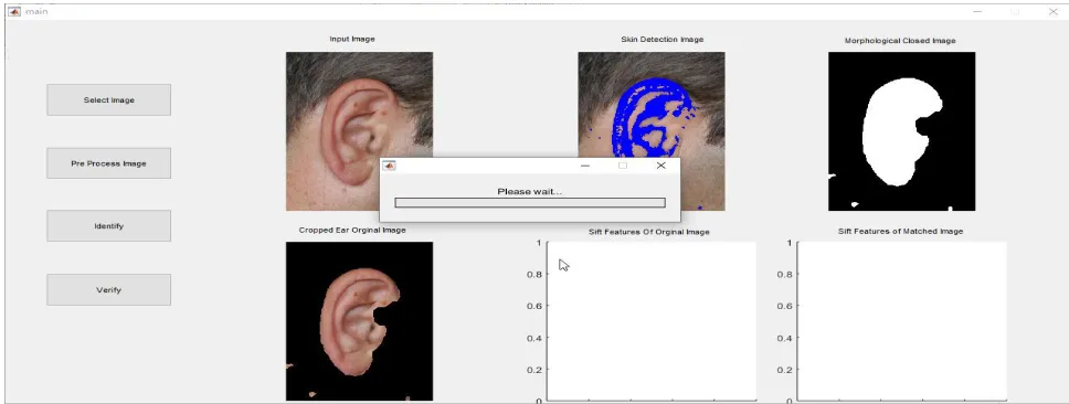
RESULTS
The study results shows that the efficient
working of ear identification and
verification system. The results under go
three stages of operations: Ear
Extraction using Skin detection by
YCBCR color space algorithm, Ear
Detection using Morphological Closing
image, Ear Identification and
verification using SIFT (Scale-invariant
feature transform) and EDM (Euclidean
P a g e | 5363
Figure 3: Ear input
In the first stage of process the system takes a ear image as input image and under goes
process.
Figure 4: Ear extraction using skin detection
The second stage of the process is
identification of ear from the input
image using skin detection system by
Ycbcr color space. The method analysis
the The definitions of the R', G', and B'
signals also differ between BT.709 and
BT.601, and differ within BT.601
depending on the type of TV system in
use (625-line as in PAL and SECAM or
525-line as in NTSC), and differ further
in other specifications. In different
definitions of the R, G, and B
chromaticity coordinates, the reference
white point, the supported gamut range,
the exact gamma pre-compensation
functions for deriving R', G' and B' from
R, G, and B, and in the scaling and
offsets to be applied during conversion
from R'G'B' to Y′CbCr. So proper
conversion of Y′CbCr from one form to
the other is not just a matter of inverting
one matrix and applying the other. In
fact, when Y′CbCr is designed ideally,
the values of KB and KR are derived
from the precise specification of the
RGB color primary signals, so that the
luma (Y′) signal corresponds as closely
as possible to a gamma-adjusted
measurement of luminance (typically
based on the CIE 1931 measurements of
the response of the human visual system
to color stimuli).
Figure 5: Ear Extraction using morphological close image
In the third procedure the ear
extraction is done utilizing
morphological close picture handling
strategy. Where by the playing out a
disintegration on the picture after the
expansion, i.e. an end, we lessen some of
this impact. The impact of shutting can
be effectively imagined. Envision taking
the organizing component and sliding it
P a g e | 5365
without changing its introduction. For
any foundation limit point, if the
organizing component can be made to
touch that point, with no part of the
component being inside a frontal area
district, then that point remains
foundation. In the event that this is
impractical, then the pixel is set to closer
view.M2 = imclose(IM,SE) performs
morphological closing on the grayscale
or binary image IM, returning the closed
image, IM2. The structuring element,
SE, must be a single structuring element
object, as opposed to an array of objects.
The morphological close operation is a
dilation followed by erosion, using the
same structuring element for both
operations. IM2 = imclose(IM,NHOOD)
performs closing with the structuring
element strel(NHOOD), where NHOOD
is an array of 0's and 1's that specifies
the structuring element neighborhood.
gpuarrayIM2 =
imclose(gpuarraryIM,___) performs the
operation on a graphics processing unit
(GPU), where gpuarrayIM is a gpuArray
containing the grayscale or binary
image. gpuarrayIM2
is a gpuArray of the same class as the input image.
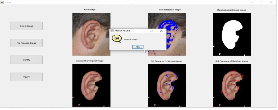
In the fourth stage, after the ear
identification process we move to ear
identification process. Here the image is
identified by matching the input image
using SIFT and EDM method. SIFT
keypoints of objects are first extracted
from a set of reference images and
stored in a database. A object is
perceived in a new image by exclusively
contrasting every element from the new
image to this database and discovering
applicant coordinating elements in light
of Euclidean separation of their element
vectors. From the full arrangement of
matches, subsets of keypoints that
concur on the question and its area,
scale, and introduction in the new
picture are distinguished to sift through
great matches. The assurance of
predictable clusters is performed quickly
by utilizing a productive hash table
usage of the summed up Hough change.
Every bunch of at least 3 includes that
concur on a protest and its posture is
then subject to assist point by point
display confirmation and in this manner
exceptions are disposed of. At last the
likelihood that a specific arrangement of
components demonstrates the nearness
of a question is registered, given the
precision of fit and number of plausible
false matches. This is a quick strategy
for giving back the closest neighbor with
high likelihood, and can give speedup by
element of 1000 while finding closest
P a g e | 5367
Figure 7: Ear Verification
By using the above explained SIFT and
EDM the image verification process is
carried in Matlab [14].
CONCLUSION
In this paper, an ear Identification System
based on images is proposed. The primary
commitments of the proposed strategy are
the accompanying: (1) Ear Extraction
utilizing Skin detection by YCBCR shading
space calculation, Ear Detection utilizing
Morphological Closing picture, Ear
Identification and confirmation utilizing SIFT
(Scale-invariant component change) and
EDM (Euclidean Distance Measure).
Examination. Trial comes about
demonstrate that we can accomplish
programmed ear recognition in light of 2D
pictures with the proposed technique. Our
future work will be centered around two
viewpoints: (1) in the ear standardization
arrange, we have to enhance the exactness
of the ear cartilage limitation, create
ponder models for the ear cartilage historic
points, and make the seeking procedure
less subject to the underlying model shape,
and (2) in the ear authentication organize,
we require a bigger dataset to affirm the
coordinating precision and the continuous
execution of the proposed strategy.
REFERENCE
1. R.Bajcsy, and S. Lovacic,
“Multiresolution Elastic Matching,”
Computer Vision, Graphics, and
Image Processing, vol. 46, pp. 1-21,
1989.
2. S. Bochner, Lectures on Fourier
Integrals, Translated by M.
Tenenbaum, and H. Pollard,
Princeton University Press,
Princeton, New Jersey, 1959.
3. J. Canny, “A Computational
Approach to Edge Detection,” IEEE
Trans. Pattern Analysis and Machine
Intelligence, vol. 8, no. 6, pp.
679-698, 1986.
4. D.P. Huttenlocher, G.A.
“Comparing Images Using the
Hausdorff Distance,” IEEE Trans.
Pattern Analysis and Machine
Intelligence, vol. 15, no. 9, pp.
850-863, Sep. 1993.
5. Wolfram, A., Fussel, D., Brune, T.,
& Isermann, R. (2001).
Component-based multi- odel approach for fault
detection and diagnosis of a
centrifugal pump. In American
Control Conference, 2001.
Proceedings of the 2001 (Vol. 6, pp.
4443-4448). IEEE.
6. Boukhris, A., Mourot, G., & Ragot,
J. (1999). Non-linear dynamic
system identification: a multi-model
approach. International Journal of
Control, 72(7-8), 591-604.
7. Lu, L., Zhang, X., Zhao, Y., & Jia,
Y. (2006, August). Ear recognition
based on statistical shape model. In
First International Conference on
Innovative Computing, Information
and Control-Volume I (ICICIC'06)
(Vol. 3, pp. 353-356). IEEE.
8. Mazinan, A. H., & Sadati, N. (2010).
Fuzzy predictive control based
multiple models strategy for a
tubular heat exchanger system.
Applied Intelligence, 33(3), 247-263.
9. Cen, Z., Wei, J., & Jiang, R. (2013).
A gray-box neural network-based
model identification and fault
estimation scheme for nonlinear
dynamic systems. International
journal of neural systems, 23(06),
1350025.
10.Schulte, H., & Hahn, H. (2001).
Identification with blended
multi-model approach in the frequency
domain: an application to a servo
pneumatic actuator. In Advanced
Intelligent Mechatronics, 2001.
Proceedings. 2001 IEEE/ASME
International Conference on (Vol. 2,
P a g e | 5369
11.Yan, P., & Bowyer, K. W. (2006,
June). An Automatic 3D Ear
Recognition System. In 3DPVT (pp.
326-333).
12.Aibinu, A. M., Salami, M. J. E.,
Shafie, A. A., Hazali, N., &
Termidzi, N. (2011, January).
Automatic fruits identification
system using hybrid technique. In
Electronic Design, Test and
Application (DELTA), 2011 Sixth
IEEE International Symposium on
(pp. 217-221). IEEE.
13.Yan, P. (2006). Ear biometrics in
human identification (Doctoral
dissertation, University of Notre
Dame).
14.Charfi, N., Trichili, H., Alimi, A. M.,
& Solaiman, B. (2016). Bimodal
biometric system for hand shape and
palmprint recognition based on SIFT
sparse representation. Multimedia