Quantitative measurements of feature indexing for 2D binary images of hexagonal grid for image retrieval

(1)

VICTORIA

~

UNIVERSITY

•

... ~

"

z

0

~

0

~

DEPARTMENT OF COMPUTER AND

MATHEMATICAL SCIENCES

Quantitative Measurements of Feature Indexing

for 2D Binary Images of Hexagonal

Grid for Image Retrieval

Z. J

.

Zheng and C. H

. C

. Leung

(51COMP18)

February, 1995

(AMS

: 63H30

, 68P20, 68Ul0)

TECHNICAL REPORT

VICTORIA UNIVERSITY OF TECHNOLOGY

(P

0 BOX 14428) MELBOURNE MAIL CENTRE

MELBOURNE, VICTORIA,

3000

AUSTRALIA

TELEPHONE (03) 9688 4249

I

4492

(2)

Quantitative Measurements of Feature Indexing for 2D Binary Images of Hexagonal Grid for Image Retrieval

Z.J. Zheng and C.H.C. Leung

Department of Computer and Mathematical Sciences, Victoria University of Technology PO Box 14428, Vic. 3000, Australia

ABSTRACT

A new feature indexing scheme for binary images is proposed. Using the structures of the conjugate classifi-cation of the hexagonal grid, ten intrinsically geometric invariant clusters are identified to partition a binary image into ten feature cluster images. The numbers of feature points in feature images are evaluated. Using the ten integers, a probability model is defined to generate quantitative measurements for feature indexing. This provides intrinsic feature indexing sets for rapid retrieval images based on their contents. Two vectors of twelve probability measurements are used to describe different images in varying sizes and sample pictures and thire feature indices are illustrated.

Keywords: Structural Classification, Intrinsically Geometric Invariant, Pattern Recognition, Visual Infor-mation Management, Image Retrieval, Automatic Indexing

1 Introduction

1.1 Visual Information Management

Human information processing often involves the recognition, storage, and retrieval of images and pictorial information. Although large numbers of images are generated and used everyday, current information systems are incapable of dealing with them efficiently, as these systems are primarily designed to function with symbolic and structured data. While there is no difficulty for humans to flexibly recognize and retrieve the contents in an image, this presents severe difficulties for current computers. To effectively exploit Pattern Recognition, Computer Vision and Visual Information Management Systems (VIMS) [1], it requires new techniques for feature representation and data management, and images must be suitably organized for rapid retrieval based on their contents.

1.2 Problem

It is widely accepted that efficient feature indexing is central to any successful VIMS implementa-tion. Such indexing may be automated in varying degrees, and a number of researchers have been interested in this issue. Using object partitioning, Oommen and Fothergill [2] proposes an auto-matic indexing scheme for image databases, where the task is not merely viewed as recognition or classification, but instead as one of partitioning the image set in terms of their visual resemblances. A key problem they identify is that of partitioning the images into unequal size sub-databases.

2 A New Scheme

(3)

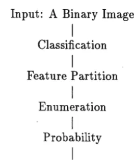
Input: A Binary Image

I

Classification

Feature Partition

Enumeration

Probability

I

Output: Two Vectors of Feature Indexing

Figure 1: Procedure of Feature Indexing

binary images [4] ( n images representing 0 feature points and. another n images representing 1 feature points). It is convenient to use a specific scheme of the conjugate classification using three parameters. Using this scheme, the set of entire patterns can be classified into 22 classes. After the operation of classification, a feature image composed of three parameters for each point can be generated from the initial image. Repartitioning these feature classes into ten feature clusters and applying the partition to the feature images, the numbers of points in ten feature clusters can be calculated respectively. These clusters represent "Inner, Block Edge, Line Connection, Intersection and Noise" points for 1 and 0 values respectively. Ten numbers of these feature points can retain invariance under the transportation, rotation and reflection operations on the initial image.

The organization of this paper is as follows. The procedure of feature indexing is shown in Figure 1. The conjugate classification are explained in section 3. The feature partition of ten feature clusters is introduced in section 4. The enumeration is formulated in section 5. Probability and two vectors of feature indexing are defined in section 6. To show the usefulness of our proposal, four sets of sample images and their feature indices are illustrated in section 7 and finally the main application areas of the proposal are discussed in section 8.

3 Classification

3.1 Kernel Form of Hexagonal Grid

Let X denote a binary image on the hexagonal grid, x E X be a given point of the image. The simplest scheme for feature indexing on the hexagonal grid uses seven adjacent grid points (the kernel form of the hexagonal grid) as the structuring form. The kernel form is a regular form composed of seven grid points for which one point x is at the centre and another six neighbouring points

x

0 -

x

5 are around it. The kernel form can be denoted by

K(x)

shown in Figure 2. Each

(4)

K(x)= xs

x x2 =

(x, xs,

···,Xi,···, x1, x0 ) =

(x

6 ,

x

5 , ···,Xi,···, x 1,

x

0 ),

Xi E {0, l}, 0::::;

i::::;

6, x EX.

Figure 2: The Kernel Form of the Hexagonal Grid

3.2 Conjugate Classification of Kernel Form

The conjugate classification of the kernel form of the hexagonal grid is established by Zheng and Maeder [3] and further systematic investigations are shown in Zheng [4,5]. For a convenient de-scription, the classification can be briefly described as follows.

The kernel form K ( x) of the hexagonal grid is a point x with six neighbouring points around it. When each point is allowed to assume values of only 0 or 1, there is a total of 128 states corresponding to unique instances of the kernel form. From the state set

y(K(x)) of 128 states and

the inclusion relation of set theory, one can use a hierarchy of six levels to represent the conjugate classification. Each level contains 128 states and each node is a subset of states. Any two nodes in the same level do not contain the same state. If one lets Q(K(x )) be the root, then the first level can be divided into one state set G and one conjugate state set G dependent on the value of the centre point x, x E {O, l}. The second level of 14 nodes {pG,p

G}

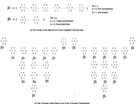
can be distinguished by p, the number of connections, 0 ::::; p ::::; 6, that is, the number of six neighbouring points with the same value of the centre point. The third level of 22 nodes

HG}

and {~G} is related to q which corresponds to the number of branches, 0 ::::; q ::::; 3 (the number of runs of the six neighbouring points with the same value of the centre point in each state). The fourth level of28 nodes {~Gs} and {~Gs} has the property of rotational invariant in which any two states in a node can be congruent by rotation, and s denotes the number of spins, s E {-1, 0, 1}. Only six nodes for q = 2 need to be identified using

s. The fifth level of 128 leaves {~G~} and {iG~} has a simple relation to the respected state, and

r denotes the number of rotations 0 ::::; r ::::; 5. In short, the conjugate classification is a hierarchy of six levels: one root, two nodes, 14 nodes, 22 nodes, 28 nodes and 128 leaves. Each node of the hierarchy is a class of states with 1-5 calculable parameters. The symbols ( x, p, q, s, r) are used to denote five calculable parameters of this classification. For convenience, each intermediate node can be called a class.

3.3 Proper Level for Feature Indexing

The hierarchical structure of the conjugate classification provides a flexible framework for support-ing different applications. It is obvious for our purpose that x or (x,p) is not sufficient for describing the intrinsically geometric invariant clusters. It is necessary to use three parameters ( x, p, q) for the description.

(5)

1 1 0 1 0 0 1 0 1 1 1 1 _{X6= 1,}

lG

= 0 1 1 0 1 1 1 1 1

' 1 1 0 1 1 0 1 1 1 } p = 4, four connections;

0 1 1 1 1 1 1 1 1 0 0 0

q = 1, one branch.

~ 0 1 1 0 X6=0;

= 1 0 0 0 0 1 }

0 1 1 0 p = 3, three connections;

q = 3, three branches.

(a) Two Nodes of lbe 1birdLevel of lbe Conjugale Classification

0 0 1 1 1 1 0 0

0 1 0 1 1 1 1 0 1 0 0 0

0 0 1 1 1 1 0 0

gG 1 0 1 1 1 1 1 1 1 1 ~G gG 0 1 0 0 0 0 0 0 0 0 ~G 0 1 0 0 1 0 0 1 1 0 1 1 0 1 1 1 0 1 1 0 1 1 0 0 1 0 0 1 0 0

0 0 0 0 0 0 0 1 1 1 1 1 1 1 1 1 1 0 0 0

JG ~G ~G

!G

~G 1 1Q ~G ~G

!G

~G

1 0 1 0 1 0 0 1 0 1 0 1

0 1 1 0 1 1 0 1 1 1 0 0 1 0 0 1 0 0

0 0 0 1 1 1 1 1 1 0 0 0

1 0 1 0 1 1 0 1 0 1 0 0

0 1 0 0 1 0 0 1 0 1 0 1 1 0 1 1 0 1

0 1 1 1 1 1 1 0 0 0 0 0

~G ~G ~ _~ ~G 2Q

4

1 0 0 1

0 1 1 1 0 0

1 0 0 1

~G _~

(b) The 22 Nodes of lbe Third Level of Ille Conjugale Classification

Figure 3: The Third Level of the Conjugate Classification

4 Feature

Partition

4.1 Conjugate

Partition of Ten

Feature Clusters

0 0 3 o-o-

3-For convenient description, 22 feature classes {₀G, ₆G, ... ,₃G} and {₀G, ₆G, ... ,₃G} can be symbol-ized as letters {A, B, ... , K} and {a, b, ... , k} representing classes in two pseudo-triangles respectively in Figure 4.

These classes can be reorganized into ten intrinsically geometric invariant clusters defined and symbolized as follows:

A

1-lnner Cluster =

C D E F G

H I J

K

B a

{B};

c d e f g

h J

k

Figure 4: Symbolized Two Pseudo-Triangles

(1)

(6)

~

C1

=

0-Inner Cluster

=

{b };

(2)

C2

=

1-Block Edge Cluster

=

{D,E,F,G};

(3)

C2

=

0-Block Edge Cluster

=

{d,e,f,g};

(4)

C3

=

1-Line Connection Cluster

=

{H,K};

(5)

C3

=

0-Line Connection Cluster

=

{h,k};

(6)

C4

=

1-lntersection Cluster

=

{J,J};

(7)

C4

=

0-lntersection Cluster

=

{i,j};

(8)

Cs

=

1-N oise Cluster

=

{A,C};

(9)

Cs

=

0-N oise Cluster

=

{a, c}. (10)

5 Enumeration

For any point

x

E X, the conjugate classification generates a corresponding feature point G(

x)

=

(x,p,q).

Applying this procedure to

Vx

EX, a feature image denoted by

G(X)

=

(X,P,Q)

is

evaluated from the initial image X. Because each feature point G( x) has to belong in one of

feature clusters either in

{Ci}

or {

C:}.

This relationship can be used to enumerate ten numbers

of feature points for corresponding specific feature clusters. A projective operation can be defined

and denoted by

T(. ).

Let

Tc(G(x))

= {

~:

where C indicates one feature class.

ifG(x)EC;

otherwise (11)

Undertaking the projective operation, ten integers

{Ni}

and

{Ni}

can be generated;

conse-quently:

Ni

L

Tc,(G(x)), 1 :::;

i:::;

5; (12) 'v'G(x)

Ni

L

Tc;(G(x)), 1:::;

i:::;

5; (13) 'v'G(x)

6 Probability and Feature Indexing

Using the ten integers, a probability model can be defined to represent feature indexing vectors in a normalized form. Owing to the direct correspondence among 1 and 0 feature points between clusters and enumerated values, more parameters can be deduced. Summarizing total numbers of 1 and 0 points, there are the following equations:

s

N = LN··

i,

(14)

i=l s

fe

l:fei;

(15)

i=l

Po N/(N

+

N);

(16)

(7)

Po+ Po

1·

'

Pi

Ni/N, Pi

2::

0, 1 :::; i :::; 5;

Pi

Ni/N,

Pi

2::

o,

1 :::; i :::; 5;

LPi

= 1.

In convention, two vectors of feature indexing are defined as

(po : Pl' P2, p3, p4, Ps)

(Po

:

Pi,

P2,

fo,

p4,

Ps)

for 1 feature indexing and

for 0 feature indexing.

(18)

(19)

(20)

(21)

(22)

(23)

Following this procedure, the ten integers are generated as twelve measurements of probability in two vectors. Each probability measurement indicates the specific strength of the feature cluster in the processed image. Their values are intrinsically dependent on their contents. Because the structure of feature cluster can retain invariant properties under multiple geometric transforma-tions: transportation, rotation and reflection, it is possible to use feature indexing to collect a set 0f intrinsically geometric invariant images in an equivalent collection directly.

Using this probability model, any binary image can be transformed into two vectors with a total of twelve components. It provides a unified framework to support further representing, organizing, retrieving and manipulating of binary images based on their intrinsical contents.

7 Sample Images and Their Measurements

To show the usefulness of proposed scheme, four sets of sample pictures are selected. Nine pictures (a )-(i) and their feature indices are listed in Appendix A. Picture (a) is a binary image of Lenna in 512x512. Twelve integers of N,

N,

{Ni}

and

{Ni}

are listed under the picture. Two vectors of feature indexing are also presented. Picture (b) is an edge image of picture (a). Its 1 feature indexing indicates the image dominated by 1-line components. Picture ( c) is a binary mandrill image, its feature indexing has significant difference from picture (a). Pictures ( d) and ( e) are two pictures in different sizes (a) in 512x256 and (b) in 256x256. However they are composed of similar kinds of components. It is interesting that their feature indices are similar too. Two line dominant images are shown in Picture (f) and Picture (g). (f) is a 0-line image and (g) is a 1-line image. Picture (h) and Picture (i) are two complementary images. Two vectors of their feature indices are just exchanged each other. From these pictures and their feature indexing, it is possible to organize different images in order to provide a new way to manage and retrieval image information by its contents. The proposed scheme provides additional information of intrinsically geometric components in the image.

8 Conclusion

(8)

REFERENCES:

l. R. Jain (ed.), NSF workshop on Visual Information Management Systems, SIGMOD RECORD,

Vol.22, No. 3, pp57-75, 1993

2. J. Oommen and C. Fothergill, Fast !Learning Automaton-based Image Examination and Retrieval, The Computer Journal, Vol. 36, pp. 542-553, 1993

3. Z.J. Zheng and A.J. Maeder, The Conjugate Classification of the Kernel Form of the Hexag-onal Grid, in Modern Geometric Computing for Visualization, Eds by T.L. Kunii and Y. Shinagawa, pp73-89, Springer- Verlag, 1992

4. Z.J. Zheng and A.J. Maeder, The Elementary Equation of the Conjugate Transformation for Hexagonal Grid, Modeling in Computer Graphics, Eds by B. Falcidieno and T.L. Kunii, pp21-42, Springer- Verlag, 1993

(9)

Appendix A

0-Pixels 1-Pixels SUM Total: 50074 80998 131072

Inners: 38998 70396 B-edges: 9593 8909 Lines: 328 429 Inters: 749 732 Noises: 406 532

0 Feature Indexing:

(0.3820 : 0.7788, 0.1916, 0.0066, 0.0150, 0.0081} 1 Feature Indexing:

(0.6180 : 0.8691, 0.1100, 0.0053, 0.0090, 0.0066}

0 Feature Indexing:

(0.9232: 0.8598, 0.1298, 0.0026, 0.0034, 0.0043} 1 Feature Indexing:

(0.0768 : 0.0000, 0.1349, 0.6989, 0.1523, 0.0139}

Total:

Inners:

B-edges: Lines:

Inters:

Noises:

(b)

0-Pixels 1-Pixels 66091 64981 30078 32153 24677 2047.8 2575 2972 5744 5813 3017 3565 0 Feature Indexing:

SUM 131072

(0.5042 : 0.4551, 0.3734, 0.0390, 0.0869, 0.0456} 1 Feature Indexing:

(0.4958 : 0.4948, 0.3151, 0.0457, 0.0895, 0.0549}

(c)

Inners: 16894 17323 B-edges: 15026 15254 Lines: 132 119 Inters: 321 315

Noises: 74 78 0 Feature Indexing:

{0.4951 : 0.5207, 0.4631, 0.0041, 0.0099, 0.0023} 1 Feature Indexing:

(0.5049 : 0.5235, 0.4610, 0.0036, 0.0095, 0.0024} (d)

Inners; 8607 8642 B-edges: 7470 7504

Lines: 76 59 Inters: 178 145

Noises: 37 50 0 Feature Indexing:

(0.4995: 0.5258, 0.4564, 0.0046, 0.0109, 0.0023} 1 Feature Indexing:

(0.5005 : 0.5270, 0.4576, 0.0036, 0.0088, 0.0030}

(e)

Figure 5: Sample Pictures and Measurements Sizes of Original Pictures

(a), (b), (c): 512x512 ( d) : 512x256

(10)

0 Fea.ture Indexing:

(0.2400 : 0.0000, 0.0698, 0.7940, 0.1362, 0.0000)

(0.7600 : 0.4736, 0.4910, 0.0083, 0.0154, 0.0117)

(f)

O Fea.ture Indexing:

(0.8318 : 0.6273, 0.3447, Q.0222, 0.0014, 0.0044)

(0.1682: 0.0000, 0.0278, 0.8809, 0.0911, 0.0002)

(g)

0 Feature Indexing:

(0.7426: 0.7508, 0.2286, 0.0051, 0.0061, 0.0095)

1 Feature Indexing:

(0.2574 : 0.2650, 0.6385, 0.0763, 0.0202, 0.0000)

(h)

0 Feature Indexing:

(0.2574 : 0.2650, 0.6385, 0.0763, 0.0202, 0.0000)

1 Feature Indexing:

(0.7426 : 0.7508, 0.2286, 0.0051, 0.0061, 0.0095)

(i)

Figure 6: Sample Pictures and Feature Indexing Sizes of Original Pictures in 256x256

(f) 0 line components (g) 1 line components (h) 1 objects

(11)