An Approach for Vehicle Detection in Complex Environments
Dimple Chawla
Assistant Professor, Delhi Institute of Advanced Studies
Abstract
This paper presents an approach for vehicle detection in complex environments such as sunny days, rainy days, cloudy days, sunrise time, sunset time, or night time. The vehicle detection under various environments will have many difficulties such as illumination vibrations, shadow effects, and vehicle overlapping problems that appear in traffic jams. The main contribution of this paper is to propose an adaptive vehicle detection approach in complex environments to directly detect vehicles without extracting and updating a reference background image in complex environments. In the proposed approach, histogram extension addresses the removal of the effects of weather and light impact. The gray-level differential value method (GDVM) is utilized to directly extract moving objects from the images. Finally, tracking and error compensation are applied to refine the target tracking quality. In addition, many useful traffic parameters including traffic flows, velocity, and vehicle classification are evaluated that can help to control traffic.
Keywords: Histogram Extension (HE), tracking compensation, tracking, traffic jam, vehicle detection.
1. Introduction
In Today’s Era as the numbers of vehicles are increasing, related traffic information becomes
very important for drivers. Vehicle detection is an important problem in many related
applications, such as self-guided vehicles, driver assistance systems, intelligent parking systems, or measurement of traffic parameters, like vehicle count, speed, and flow. One of most common approaches to vehicle detection is using vision-based techniques to analyze vehicles from images or videos. However, due to the variations of vehicle colors, sizes, orientations, shapes, and poses, developing a robust and effective system of vision-based vehicle detection is very challenging.
Wang [2] proposed a joint random field (JRF) model for moving vehicle detection in video sequences. The proposed method could handle moving cast shadows, lights, and various weather conditions. However, the method did not recognize vehicle classification and velocity. Tsai et al. [3] presented a novel vehicle detection approach for detecting vehicles from static images using color and edges. This method introduced a new color transform model to find important “vehicle color” for quickly locating possible vehiclecandidates. This method could also detect vehicles in various weather conditions, but it did not address resolutions on traffic jams and shadow reduction. Zhang et al. [4] developed a multilevel framework to detect and handle vehicle occlusion. The proposed framework consisted of intraframe, interframe, and tracking levels to resolve the occluded vehicles. Neeraj et al. [5] gave a method for segmenting and tracking vehicles on highways using a camera that was relatively low. Melo [6] described a low-level object tracking system that produced accurate vehicle motion trajectories, which could further be analyzed to detect lane centers and classify lane types. A lane-detection method that was aimed at handling moving vehicles in traffic scenes was proposed by Cheng et al. [7]. A new background subtraction algorithm based on the sigma–delta filter, which was intended to be used in urban traffic scenes, was presented in [8]. An example-based algorithm for moving vehicle detection was introduced in
[9]. In addition, many approaches have been proposed for tackling related problems in ITS. The model based approach [10] uses a 3-D model to detect vehicles. In this method, different models that correspond to different types of vehicles are created. Song et al. [11] and Koller et al. [12] used an active contour method to track vehicles. In this method, the vehicles could easily be tracked, and computation loading could significantly be reduced. However, system initialization was a critical risk. Coifman [13] developed a vision-based system with gradient operator to detect subcorner features of the vehicles and grouped these features to detect the vehicles. The advantage of this method was that it was less sensitive to change in illumination. On the other hand, this method could meet the challenge of determining grouping conditions. Wang et al. [14], detected the motion information of the spatial– temporal wavelet of video sequence. Cucchiara et al. [15] integrated moving edge detection and headlight detection into a hybrid system. This system worked not only during the day but also at night. Unlike most methods referring to background image, they used a three-image difference to detect moving edge. This method reduced both the dependence on background and the time of background learning. However, noise affected the system to a great extent. Background segmentation was one approach for extracting the common part between different images in a frame. With good flows of learning and updating, objects could more completely be extracted. Beymer et al. [16] proposed a vehicle-tracking algorithm to estimate traffic parameters using corner features. In addition, Liao et al. [17] used entropy as an underlying measurement to calculate traffic flows and vehicle speeds. Baker et al. [18] proposed a 3-D model matching scheme to classify vehicles into various types, such as
wagons, sedan, and hatchback. Furthermore, Gupte et al. [19] proposed a region-based
approach to track and classify vehicles based on the establishment of correspondences between regions and vehicles. In [16], [19], and [20], a manual method of camera calibration has been presented to identify lane locations and corresponding lane widths.
In this paper, an adaptive vehicle detection approach for complex environments is proposed for solving problems of vehicle detection in traffic jams and complex weather conditions like sunny days, rainy days, sunrise, sunset, cloudy days, fog, or at night. Histogram extension (HE) addresses how we can remove effects of weather and light impact. The gray-level differential value method (GDVM) is used to dynamically segment moving objects. Finally, tracking and error compensation are applied to refine the target tracking quality. In addition, many useful traffic parameters are evaluated from the proposed approach, including traffic flows, velocity, and vehicle classifications. These useful parameters can help in controlling traffic and provide drivers good driving guidance.
This paper is organized as follows. Section II addresses the system overview. Section III shows the HE method, which makes images from various environments similar to each other. Dynamic moving object segments, including GDVM and the tracking procedure, are presented in Section IV and V. Finally, experimental results are given in Section VI, and the conclusion is presented in Section VII.
II. SYSTEM OVERVIEW
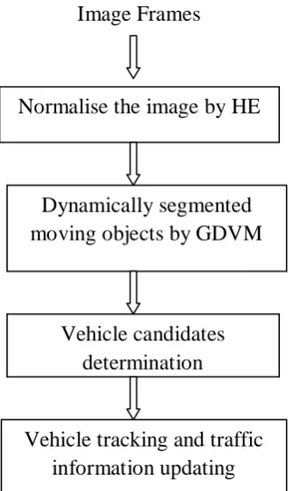
Fig.(1) shows the system overview of the proposed approach. There are several steps in the flowchart. The image frames taken from the video are first normalised using the Histogram Extension (HE) technique. Then moving objects are dynamically segmented using GDVM. Next, vehicle detection, vehicle tracking, and error compensation are applied. Finally traffic
parameters are evaluated and updated. To reduce the computing load all methods are applied only in the region of interest (ROI) shown in fig.(2)
Fig. (2) Source image and its ROI
Fig .(1) System overview of proposed method
III. HISTOGRAM EXTENSION
In histogram extension (HE) method, first decompose a true color image into its red–green– blue (RGB) components and then calculate the histogram in the region of interest (ROI) for each RGB component. After that, linear normalization with mean shift (LNMS) is applied to normalize the source images. In LNMS method,
(i) the original mean value of all pixels, denoted as mp is shifted to 128 as given by
equation (1).
𝑚𝑝 = ∑ 𝑖 255
𝑖=0 ∗ 𝑠(𝑖)
∑255𝑠(𝑖)
𝑖=0 … (1)
(ii)Next, α and β, which are defined as shifting parameters are calculated for the left and right zones given by equation (2) & (3)
𝛼 = 128
𝑚𝑝 (2)
𝛽= 255128− 𝑚
𝑝 (3)
(iii) Finally, all gray levels that correspond to gray-level counts, denoted as iL(s) in the left
zone and iR(s) in the right zone, are normalized to the new ones, denoted as niL(s) and niR(s)
given by equation (4) & (5) Image Frames
Normalise the image by HE
Dynamically segmented moving objects by GDVM
Vehicle candidates determination
Vehicle tracking and traffic information updating
𝑛𝑖𝐿(𝑠) = 𝑖𝐿(𝑠)∗ 𝛼 … (4)
𝑛𝑖𝑅(𝑠) =𝑖𝑅(𝑠)∗ 𝛽 … (5)
The LNMS method is explained below as shown in fig.(3)
Fig.(3) LNMS Fig.(4) Histogram Extension
When LNMS is applied to each component of RGB, the mean values of R, G and B will approach 128. Also, the gray level scale in the left zone is smoothly normalized to 0 and 128, and the gray level scale in the left zone is smoothly normalized to 128 and 255.
Thus, Histogram Extension (HE) is a method that removes the effect of weather and light impact as it makes the histogram normalized i.e. equally distributed. This benefit simplifies system parameter setting, noise reduction and moving object segments.
The effect of histogram extension is shown in fig.(4). As we seen that the darker areas in original image get lighter after applying histogram extension so that we easily clear the objects in the image.
IV. DYNAMICALLY MOVING OBJECT SEGMENT AND TRACKING PROCEDURE
In a vehicle detector, the desired moving objects should be segmented from the road surface. To segment the correct moving objects fast without using background concepts. For this Gray differential value method (GDVM) is used. GDVM among the R, G and B components is applied in the proposed system. Vehicle candidates can be extracted from the moving objects by merging fractal objects or splitting mismerged objects. Then, a tracking procedure is used to guarantee the detection quality, including filter noises. Finally, to improve the accuracy of traffic parameters and ensure the stability of the tracking flow, a tracking compensation method is used.
(A)Dynamically Segmenting Moving Objects by GDVM
It is used to segment moving objects from the background. Gray road surfaces and white or yellow lane marks are assumptions in GDVM while the remaining colors are taken as moving objects on the road. To extract gray like cars, because the luminance (Y) of white cars is higher and the Y of dark cars is lower than the road surface, the Y value of the road surface always locates by excluding the range between the two threshold values. The green component (G) of the RGB model contributes around 60% to Y. Therefore, the G value can be adopted to reduce the computational loading and gray like cars can be segmented by
compensating for the moving objects. For gray, white and yellow, ΔRG, ΔRB and ΔGB are
small given by equation (6), (7) and (8)
∆𝑅𝐺(𝑥,𝑦) = |𝑅(𝑥,𝑦)− 𝐺(𝑥,𝑦)| (6)
∆𝑅𝐵(𝑥,𝑦) = |𝑅(𝑥,𝑦)− 𝐵(𝑥,𝑦)| (7)
∆𝐺𝐵(𝑥,𝑦) = |𝐺(𝑥,𝑦)− 𝐵(𝑥,𝑦)| (8)
In practical cases, most non-gray cars, including white and black cars, can be segmented by equation (9) 𝑀𝑂 (𝑥,𝑦) = ⎩ ⎪ ⎪ ⎨ ⎪ ⎪ ⎧ 1
∆𝑅𝐺(𝑥,𝑦) >𝑇𝐻𝑅𝐺𝑎𝑛𝑑
∆𝑅𝐵(𝑥,𝑦) >𝑇𝐻𝑅𝐵𝑎𝑛𝑑
∆𝐺𝐵(𝑥,𝑦) >𝑇𝐻𝐺𝐵𝑜𝑟 (𝑇𝐻𝑙𝑜𝑤 ≥ 𝐺(𝑥,𝑦)𝑜𝑟
𝐺(𝑥,𝑦)≥ 𝑇𝐻ℎ𝑖𝑔ℎ) 0 𝑜𝑡ℎ𝑒𝑟𝑤𝑖𝑠𝑒
⎭ ⎪ ⎪ ⎬ ⎪ ⎪ ⎫ (9)
Thus, a true color image can be transformed to a binary moving object at (x,y), which is denoted as MO(x,y) in equation (9).
For calculating the thresholds THRG, THRB, and THGB for ΔRG, ΔRB, and ΔGB resp. an
adaptive thresholding procedure is used given below:
𝑓𝑅𝐺(𝑥,𝑦,𝑛) = �1, 0, ∆𝑅𝐺𝑜𝑡ℎ𝑒𝑟𝑤𝑖𝑠𝑒� (𝑥,𝑦) =𝑛 (10)
𝐷𝑅𝐺(𝑛) = � � 𝑓𝑅𝐺(𝑥,𝑦,𝑛) (11) 𝑁−1
𝑦=0 𝑀−1
𝑥=0
where, M is height of image and N is width of image.
𝐹𝐷𝑅𝐺(𝑛) =
∑𝑛+𝑝𝑖=𝑛−𝑝𝐷𝑅𝐺(𝑖)
2𝑝+ 1 (12)
where, 2p+1 is the filter order of moving average filter.
∇2𝐹𝐷
𝑅𝐺(𝑛) = 𝐹𝐷𝑅𝐺(𝑛+ 1)− 2𝐹𝐷𝑅𝐺(𝑛) + 𝐹𝐷𝑅𝐺(𝑛 −1) (13)
𝑇𝐻𝑅𝐺 = min(𝑎𝑟𝑔(𝛻2𝐹𝐷𝑅𝐺(𝑛) = 0)) (14)
Thus, THRG can be calculated by the Laplacian operator in eq.(13). Similarly, calculate other
thresholds THRB, THGB given by equation (15) & (16)
𝑇𝐻𝑅𝐵 = min(𝑎𝑟𝑔(𝛻2𝐹𝐷𝑅𝐵(𝑛) = 0)) (15)
𝑇𝐻𝐺𝐵 = min(𝑎𝑟𝑔(𝛻2𝐹𝐷𝐺𝐵(𝑛) = 0)) (16)
Now, THlow and THhigh are the thresholds for G(x,y) and they can be calculated given by the
equation (17) and (18)
𝑇𝐻𝑙𝑜𝑤 = min(𝑎𝑟𝑔(𝛻2𝐹𝐷𝐺(𝑛) = 0)) (17)
𝑇𝐻ℎ𝑖𝑔ℎ = max(𝑎𝑟𝑔(𝛻2𝐹𝐷𝐺(𝑛) = 0)) (18)
Example of applying GDVM to an image is shown in fig. (5)
(B) Detect Vehicle Candidate By Merging and Splitting Moving Objects
As we seen from equation (9) that a vehicle candidate may be broken down into several moving objects in the MO(x,y) domain. Now, it may be happen that two or more closing vehicle candidate may incorrectly be detected as one moving object. Methods of merging and splitting moving objects should be applied to more precisely detect vehicle candidates. There are several steps for these methods.
The merge boundary box rule (MBBR) is applied to merge the moving objects. The moving objects may be detected as many small rectangle boundary boxes (RBBs) in MO(x, y). MBBR is a method of merging the overlapped RBBs into a large box. When two RBBs overlap, a new RBB is rebuilt to combine and replace the two old RBBs shown in fig.(6).
Fig.(5) Example of applying GDVM .
(a) & (c) are the original image; (b) & (d) are the segmented result
Fig.(6) Example of MBBR by merging RBBs
After applying MBBR, fractal moving objects are merged as more solid ones, as shown in Fig. (7). To determine whether a vehicle candidate or not is determined by several attributes like width, height, width/height ratio, and density of moving object. When moving objects have suitable attributes, they are identified as vehicle candidates. Otherwise, they are further merged or split.
When a vehicle is broken into several moving objects, some conditions should be met. 1. The adjacent moving objects should have similar width and density.
2. The two moving objects should be shown as close.
3. The new merged moving object should have suitable attributes, including width,
height, and density.
Fig. (8) Vertical projection gap between closing objects
Fig. (7) Example of merging fractal moving objects by MBBR
Once they meet these conditions, the moving objects should be merged as a new moving object. It may be happen that two vehicles are too close so that they mismerged as one moving object. Then they should be split into two or more moving objects. For detecting and resolving the mismerged moving objects the following steps should be followed:
(a) A mismerged moving object has improperly large height (H), width (W), H/W ratio and density. If it is a mismerged moving object, then go to next step otherwise terminated.
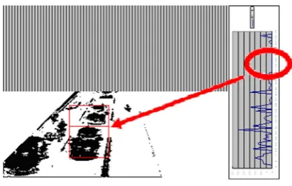
(b) If the object is mismerged then find the gap in the vertical histogram projection of the moving object shown in fig. (8). A LPF is applied to vertical histogram projection. Filtered value is given by equation (19)
𝑣𝑝∗(𝑛) = ∑ 𝑣𝑝(𝑛+𝑖) 𝑁
𝑖=−𝑁
2𝑁+ 1 (19)
where, vp(n) = histogram value at n
𝑣𝑝∗(𝑛) = filtered histogram value
Then a sliding window is used to gain the sum of the vertical histogram svp(n) at n
with 2M+1 points in equation (20)
𝑠𝑣𝑝(𝑛) = � 𝑣𝑝∗(𝑛+𝑖) (20) 𝑀
Then ssvp(n) is calculated by equation (21) which is again a sliding window.
𝑠𝑠𝑣𝑝(𝑛) = � 𝑠𝑣𝑝(𝑛+𝑖) (21) 𝑋
𝑖=−𝑋
The gap position ngap can be derived by checking the minimum ssvp(n) for all n given
by equation (22)
𝑛𝑔𝑎𝑝 =𝑎𝑟𝑔𝑛�min�𝑠𝑠𝑣𝑝(𝑛)�� (22)
(c) All moving objects and the new split moving objects should be repeatedly be checked from (a) until moving objects are evaluated.
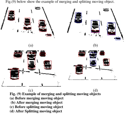
Fig.(9) below show the example of merging and splitting moving object.
V. TRACK VEHICLES WITH ERROR COMPENSATION AND UPDATE TRAFFIC PARAMETERS:
Before applying the tracking procedure, a lane mask has to be built shown in fig.(10). Meaningful traffic parameters can be updated based on the detection of the lane mask. These attributes are:
Fig. (9)Example of merging and splitting moving objects
(a) Before merging moving object (b) After merging moving object (c) Before splitting moving object (d) After Splitting moving object
1. Coordinates of the left bottom PLB and the right top PRT. The width (W), height (H)
and gravity PG of the tracked target can be gained by calculating PLB and PRT shown
by equation (23)
𝑊= 𝑃𝑅𝑇(𝑥)− 𝑃𝐿𝐵(𝑥)
𝐻 =𝑃𝑅𝑇(𝑦)− 𝑃𝐿𝐵(𝑦) (23)
𝑃𝐺 = 𝑃𝐿𝐵 +2 𝑃𝑅𝑇
Bounding box formed by PLB and PRT. A vector TA(x,y) is defined as the color value
of (x,y) in the bounding box formed by PLB and PRT. In the initial state, all pixels in
TA are set to [-1,-1,-1]. When a target is tracked, TA will be updated with equation(24)
TAn(x, y) = n−n TA1 n−1(x, y) +1n Pn(x, y) (24)
where, n is tracking count, TAn(x,y) is the color value of (x,y) at tracking count n
and Pn(x,y)is the color value in the original frame at tracking count n
2. The located lane can be used for calculating traffic information in each lane.
3. The current velocity of the tracking target is denoted as Vc = [Vcx, Vcy], and the
average velocity is denoted as VM = [VMX,VMY]which is derived by equation (25)
𝑉𝑀(𝑛) = 𝑛 −𝑛 𝑉1 𝑀(𝑛 −1) + 1𝑛 𝑉𝑐(𝑛) (25)
Vehicle tracking plays an important role in updating traffic parameters. The quality of traffic information is determined by the tracking methods. Fig. 11 shows the proposed tracking
procedure. When vehicle candidates are detected, they are correlated with the existing
tracking targets by checking the weighted determination function, denoted as DSmax [1]. If
the detected candidate has a high correlation with the existing target, the parameters of the tracking target will be updated. If the detection candidates do not correlate with any target, they will be compared with the existing tracking acquisition targets, which have yet to be identified as tracking targets. These targets may just be noise, and hence, they need to have enough tracking information to ensure that is not the case. Once targets under tracking acquisition meet adequate appearing count, new tracking targets will be created. Otherwise, the parameters of the correlated tracking acquisition target should be updated. If vehicle
Fig. (10) Setting for tracking targets. (a) Lane masks
(b) Attributes of tracked targets
candidates cannot hit any tracking or tracking acquisition targets, new tracking acquisition targets will be created.
Fig.(12) Proposed Error Compensation Fig.(11) Proposed Tracking Procedure
All undetected tracking targets should be checked if they leave the ROI. The flowchart of proposed error compensation is shown in fig. (12). When a tracking target leaves the ROI, it should be removed from the tracking list and the traffic parameters should be updated. When a vehicle is on track, its motion should not rapidly change in a short time.
If the target does not leave the ROI, the target should be redetected in the original image within a searching range based on its color transformation, denoted as TA. The searching rule is based on given equation (27) & (28)
𝑆(𝑖,𝑗) = � �|𝑓(𝑥+𝑖,𝑦+𝑗)− 𝑇𝐴(𝑥,𝑦)| 𝑦1 𝑦=𝑦0 𝑥1 𝑥=𝑥0 (27)
�𝑥𝑐,𝑦𝑐 = 𝑎𝑟𝑔𝑖,𝑗�min�𝑆(𝑖,𝑗)��� (28)
where, (xc, yc) = best predicting position in the searching range, i is the searching index for
the horizontal with searching range [-M, M], j is the searching index for the vertical with searching range [-N, N], f(x,y) is the pixel value of the original image, (x0,y0) is the left
Detect vehicle candidate
Check if the candidate are tracked targets?
Check if the candidates are tracked acquisition
targets?
Keep tracking
Check if the appearing count exceeds the tracking condition? YES YES YES NO
Check if the undetected target
leaves the ROI ?
Update traffic information
Redetect the target from original image based on predict data
Check if detect the target
Update traffic information based
on predict data
Update traffic information Create new track
bottom point and (x1,y1) is the right top point of the undetected tracking targets. An example
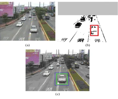
of error compensation is shown in fig. (13).
In the evaluation of traffic parameters, vehicle classification plays an important role. Basically two types of vehicle classification is there, involving large vehicles including buses and tracks and small vehicles including cars and sedans. The determination for small cars is based on equation (29)
�𝑊𝐻< 0.8< 3∗∗𝑊𝑊𝐿
𝐿 � (29)
where, W and H is the width and height of the vehicle resp. and WL is the width of the lane .
If above condition is satisfied then small vehicle otherwise large vehicle.
VI. EXPERIMENTAL RESULT
A comparison with other approaches is listed in Table II. As shown, the accuracy ratios for detecting vehicles in [1] are similar to the proposed system. However, it does not detect the vehicle velocity and vehicle classifications. The detection ratios in [14] are lower than the proposed system. In addition, it evaluates fewer traffic parameters. The detection ratios in [18] are also lower than the proposed approach. It also calculates fewer traffic parameters.
Fig. (13) Example of the error compensation procedure (a) Original image
(b) vehicle is misdetected
(c) Re-searching the vehicle in the original image
VII. CONCLUSION
An adaptive vehicle detection approach for complex environments has proposed methods for solving vehicle tracking in traffic jams and complex weather conditions, such as sunny, rain, sunrise, sunset, cloudy, or snowy days. HE is used to remove the effects of weather and light impact. The method is applied to improve the tracking accuracy ratio and simplify the system parameter settings. GDVM is used to dynamically segment moving objects. Finally, tracking and predict compensation are applied to refine the target tracking quality. The tracking accuracy ratio of the proposed system is quite good in traffic jams and complex weather conditions, particularly when applying the error compensation procedure. In the comparisons with other approaches, the proposed method not only has higher detection ratios but gathers more useful traffic parameters as well. In addition, the proposed system can easily be set up without being given any environment information in advance. Many useful traffic parameters are built, and they can be used to control the traffic. Furthermore, this information can be combined with a personal digital assistant (PDA) or mobile phone system to provide traffic conditions for vehicle drivers.
In future, some additional work can also be done to improve the accuracy ratio when it is raining and at night. Also, to make the system practical for commercial usage the detection of motorcycles is also required.
References Table II
Comparison with other approaches
(*) DC-Detection Count, TTC- Total Target Count, CR-Accuracy Ratio for vehicle classification, DCV-correct detection count for velocity
1. Bing-Fei Wu and Jhy-Hong Juang” Adaptive Vehicle Detector Approach for Complex Environment ,”IEEE Trans. Intell. Transp. Syst., vol. 13, no. 2, June 2012
2. Y. Wang, “Joint random field model for all-weather moving vehicle detection,” IEEE Trans. Image Process., vol. 19, no. 9, pp. 2491–2501, Sep. 2010.
3. L.-W. Tsai, J.-W. Hsieh, and K.-C. Fan, “Vehicle detection using normalized color And edge map,” IEEE Trans. Image Process., vol. 16, no. 3, pp. 850–864, Mar. 2007.
4. W. Zhang, Q. M. J.Wu, and X. Yang, “Multilevel framework to detect and handle
vehicle occlusion,” IEEE Trans. Intell. Transp. Syst., vol. 9, no. 1, pp. 161–174, Mar. 2008.
5. N. K. Kanhere and S. T. Birchfield, “Real-time incremental segmentation and
tracking of vehicles at low camera angles using stable features,” IEEE Trans. Intell. Transp. Syst., vol. 9, no. 1, pp. 148–160, Mar. 2008.
6. J. Melo, A. Naftel, A. Bernardino, and J. Santos-Victor, “Detection and classification of highway lanes using vehicle motion trajectories,” IEEE Trans. Intell. Transp. Syst., vol. 7, no. 2, pp. 188–200, Jun. 2006.
7. H.-Y. Cheng, B.-S. Jeng, P.-T. Tseng, and K.-C. Fan, “Lane detection with moving
vehicles in the traffic scenes,” IEEE Trans. Intell. Transp. Syst., vol. 7, no. 4, pp. 571– 582, Dec. 2006.
8. M. Vargas, J. M. Milla, S. L. Toral, and F. Barrero, “An enhanced background
estimation algorithm for vehicle detection in urban traffic scenes,” IEEE Trans. Veh. Technol., vol. 59, no. 8, pp. 3694–3709, Oct. 2010.
9. J. Zhou, D. Gao, and D. Zhang, “Moving vehicle detection for automatic traffic
monitoring,” IEEE Trans. Veh. Technol., vol. 56, no. 1, pp. 51–59, Jan. 2007.
10. D. Koller, K. Daniilidis, and H. Nagel, “Model-based object tracking in monocular image sequences of road traffic scenes,” Int. J. Comput. Vis., vol. 10, no. 3, pp. 257– 281, Jun. 1993.
11. J. C. Tai, S. T. Tseng, C. P. Lin, and K. T. Song, “Real-time image trackingfor
automatic traffic monitoring and enforcement applications,” ImageVis. Comput., vol. 22, no. 6, pp. 485–501, Jun. 2004.
12. D. Koller, J. Weber, T. Huang, J. Malik, J. Ogasawara, G. Rao, and S. Russell,
“Towards robust automatic traffic scene analysis in real-time,” in Proc. 12th Int. Conf. Comput. Vis. Image Process., 1994, vol. 1, pp. 126–131.
13. B. Coifman, D. Beyber, P. McLauchlan, and J. Malik, “A real-time computer vision system for vehicle tracking and traffic surveillance,” Transp. Res. Part C, vol. 6, no. 4, pp. 271–288, 1998.
14. Y. K.Wang and S.H.Chen, “Arobust vehicle detection approach,” in Proc. IEEE Conf. Adv. Video Signal Based Surveillance, 2005, pp. 117–122.
15. R. Cucchiara, M. Piccardi, and P. Mello, “Image analysis and rule-based reasoning for a traffic monitoring system,” IEEE Trans. Intell. Transp. Syst., vol. 1, no. 2, pp. 119– 130, Jun. 2000.
16. D. Beymer, P. McLauchlan, B. Coifman, and J. Malik, “A real-time computer vision system for measure traffic parameters,” in Proc. IEEE Conf. Comput. Vis. Pattern Recog., San Juan, PR, Jun. 1997, pp. 496–501.
17. W. L. Hsu, H. Y. Liao, B. S. Jeng, and K. C. Fan, “Real-time traffic parameter
extraction using entropy,” Proc. Inst. Elect. Eng.—Vis. Image Signal Process., vol. 151, no. 3, pp. 194–202, Jun. 2004.
18. G. D. Sullivan, K. D. Baker, A. D. Worrall, C. I. Attwood, and P. M. Remagnino,
“Model-based vehicle detection and classification using orthographic approximation,” Image Vis. Comput., vol. 15, no. 8, pp. 649–654, Aug. 1997.
19. S. Gupte, O. Masoud, R. F. K. Martin, and N. P. Papanikolopoulos, “Detection and classification of vehicles,” IEEE Trans. Intell. Transp. Syst., vol. 3, no. 1, pp. 37–47, Mar. 2002.
20. B. F. Wu, S. P. Lin, and Y. H. Chen, “A real-time multiple-vehicle detection and tracking system with prior occlusion detection and resolution and prior queue detection and resolution,” in Proc. 18th ICPR, Aug. 2006, vol. 1, pp. 828–831.