Homomorphic Encryption
?Joon-Woo Lee1, Young-Sik Kim2, and Jong-Seon No1 1
Seoul National University, Republic of Korea
2
Chosun University, Republic of Korea
Abstract. The Shell sort algorithm is one of the most practically effec-tive sorting algorithms. However, it is difficult to execute this algorithm with its intended running time complexity on data encrypted using fully homomorphic encryption (FHE), because the insertion sort in Shell sort has to be performed by considering the worst-case input data. In this paper, in order for the sorting algorithm to be used on FHE data, we modify the Shell sort with an additional parameterαand a gap sequence of powers of two. The modified Shell sort is found to have the trade-off between the running time complexity ofO(n3/2√α+ log logn) and the sorting failure probability of 2−α. Its running time complexity is close to the intended running time complexity ofO(n3/2) and the sorting failure
probability can be made very low with slightly increased running time. Further, the optimal window length of the modified Shell sort is also derived via convex optimization. The proposed analysis of the modified Shell sort is numerically confirmed by using a randomly generated ar-rays. Further, the performance of the modified Shell sort is numerically compared with the case of Ciura’s optimal gap sequence and the case of the optimal window length obtained through the convex optimization.
Keywords: Fully Homomorphic Encryption·Insertion Sort·Shell Sort
·Sorting Failure Probability.
1
Introduction
Fully homomorphic encryption (FHE) is an encryption scheme that provides encrypted data to an evaluation algorithm, which enables addition or multi-plication of plaintext without decryption. FHE enables specific operations to be performed on encrypted information without leaking any clue to the plain-text. The notion of FHE was suggested by Rivest, Adleman, and Dertouzos in 1978 [10]. Although several cryptography researchers had attempted to con-struct the FHE scheme because of its effectiveness with respect to operations in cloud systems, no one had been able to successfully construct it until 2009, when
?
Gentry succeeded in developing an FHE scheme using an ideal lattice [8]. Sev-eral researchers suggested different types of FHE algorithms in series using the bootstrapping technique in Gentry’s scheme and optimized the FHE schemes. Recently, the computation time of certain FHE schemes has been significantly reduced, which makes this scheme practically applicable. Further, the algorithms used on FHE data are expected to demonstrate the oblivious property, i.e., pro-viding the most appropriate outputs without knowing any information about the input. In other words, the behavior of an oblivious algorithm does not depend on the input data. If it depends on the input, it implies the leakage of input in-formation. The oblivious property of an algorithm is essential for FHE schemes to ensure privacy.
However, the bottleneck of operations on the FHE data is not in addition and multiplication, but involves non-arithmetic algorithms, such as sorting, search-ing, and neural networks, which are not frequently analyzed or optimized on FHE data. When processing large amounts of ciphertexts in cloud systems, it is frequently required to process the sorted data rather than unaligned data. Thus, one of the most essential non-arithmetic operations on the FHE data is the sorting algorithm, which is generally used as a subroutine algorithm of many algorithms. However, most sorting algorithms are not suitable for FHE data. For example, as the quick sort algorithm, which is one of the most popularly used sorting algorithms, is not an oblivious algorithm, it cannot be used on FHE data. Although numerous studies have been conducted to render the quick sort algo-rithm oblivious, its running time complexity becomesO(n2). Its actual running time is even longer than that of the bubble sort, which is considered to have the longest running time among all the known sorting algorithms. Therefore, modifying conventional sorting algorithms to make them suitable for FHE data is necessary. Several studies have been conducted for this purpose [1, 3, 6].
The Shell sort [11], which is one of the oldest sorting algorithms, is the generalized version of the insertion sort. The Shell sort algorithm is an in-place algorithm, which is fast and easy to implement, and thus, many systems use it as a sorting algorithm. It is known that Shell sort uses insertion sort as a subroutine algorithm, and insertion sort can be performed on the FHE data [2, 3]. However, the Shell sort should be modified to be used in the FHE setting. If we do not allow any error in sorting, then insertion sort is expected to be quite conservative, i.e., the number of operations for sorting must be set for the worst case, because the insertion sort algorithm in the FHE setting is an oblivious algorithm. Thus, if we use insertion sort in the Shell sort, the running time complexity of Shell sort in the FHE setting must beO(n2), which makes the use of Shell sort ineffective. Therefore, it is important to devise a sorting algorithm that is better than the Shell sort on the FHE data in terms of running time complexity.
It is known [2] that we can reduce the running time of insertion sort on the FHE data by allowing a sorting failure probability (SFP) using what is known as the window technique. According to this technique, in each insertion sort, instead of inserting the ith element into the subarray of (a1, a2,· · ·, ai−1), we
called the window length, immediately to the left of the ith element. We call this subarray a “window” with window lengthk.
In this paper, we devise a method to modify the Shell sort in the FHE setting using the window technique, with a running time complexity close to its original value ofO(n3/2), by deriving the running time complexity while taking the trade-off with the SFP for gap sequence 2h. It is referred to as a “modified Shell sort”. To this end, we use the exact distribution of window lengths of subarrays in each gap for successful sorting in the Shell sort. If the length of the subarray for the insertion sort in some gap iss, it is discovered that the average of the required window length for successful sorting is proportional to √s, and the right tail of its probability distribution is very thin. In the sorting process, the window length is provided as a constant multiple of√s, which ensures a negligible SFP. If the window length is close toβ√s, the SFP decays ase−β2
, which signifies a very fast-decaying function. Therefore, with a fixed negligible SFP, we can set a small window length so that the running time is asymptotically faster than that of the naive version of the Shell sort on FHE data. With this analysis, we can obtain the running time complexityO(n3/2√α+ log logn) with SFP 2−α. Thus, we can derive the trade-off between the running time complexity and the SFP using the window length and an additional parameterα.
In this paper, we address only the gap sequence of powers of two, i.e., 2h, h= 1,2,3,· · ·. Although this gap sequence is not optimal in terms of running time complexity, we first analyze the running time complexity of the modified Shell sort on FHE data, which is important for the FHE in cloud systems. The performance of the modified Shell sort is numerically compared with the cases of optimal window lengths obtained through convex optimization and Ciura’s optimal gap sequence [5], which was evaluated numerically as an optimal gap sequence in non-FHE settings. Although we do not analyze this case, the method of deriving the optimal window length in the modified Shell sort functions well for Ciura’s optimal gap sequence.
We also suggest the convex optimization method to derive a tighter window length. In other words, the window length obtained by the convex optimization method makes the running time of the modified Shell sort to be less than that of the case employing the analytical method in the modified Shell sort. This result is also numerically confirmed.
Thus, our contributions are summarized as follows:
– The exact distribution of required window length in each gap is obtained for successfully sorting each subarray in the Shell sort with the gap sequence of powers of two.
– We propose a modified Shell sort with the gap sequence of powers of two and an additional parameterαon FHE data, and derive its trade-off between the running time complexityO(n3/2√α+ log logn) and the SFP 2−α.
– The optimal window length of each gap in the modified Shell sort is derived via the convex optimization technique.
notion of FHE. In Section 3, we present the distribution of the required window length for each gap in the Shell sort on FHE data with the gap sequence of powers of two. Then, we propose a modified Shell sort for FHE and derive the trade-off between the running time complexity and the SFP. Section 4 discusses a method to deduce the optimal window length of each gap of the modified Shell sort using the convex optimization technique. Section 5 shows numerical results that support the proposed analysis. From these results, the performance in the case of the optimal gap sequence or the optimal window lengths can be observed. Section 6 concludes the study and discusses the scope for future research.
2
Preliminary
2.1 Fully Homomorphic Encryption
FHE is a public-key encryption scheme, which supports an arbitrary number of additions and multiplications of plaintext without decryption, so that anyone without the decryption key can operate the circuit with any ciphertext without leaking the information of its plaintext.
Gentry suggested the bootstrapping technique to transform homomorphic encryption to a certain degree [8], which allows only a finite number of operations on the FHE data. The bootstrapping operation has enabled several researchers to construct FHE schemes [8], which involves implementing the decryption circuit on encrypted data using the evaluation algorithm, that is, the addition and multiplication algorithms in FHE setting. All of the FHE schemes suggested thus far ensure security by adding some errors on a few elementary functions of plaintexts. As the addition and multiplication operations are repeated, the total number of errors increases, and if the total number of errors exceeds a certain limit, a decryption failure occurs. Thus, the errors need to be removed after a certain number of operations on the encrypted data, so that the ciphertexts can be further evaluated. The purpose of the bootstrapping operation is to reset the errors in the ciphertext when the errors are too large to be decrypted.
2.2 Sorting Algorithms
Although there exist several sorting algorithms [9], we consider only the insertion sort and Shell sort in this paper. These are comparison-based sorting algorithms, which do not rely on the divide-and-conquer method.
The insertion sort is an iterative sorting algorithm that sorts from the left-most element. In each iteration, we define an element to be sorted into its left-side subarray as the pivot element. It is assumed that the elements to the left of the pivot element are already sorted. We then compare the already sorted elements with the pivot element, deduce its proper position, and insert it into this posi-tion. Its worst-case and average-case running time complexities are bothO(n2). It is known that insertion sort is slightly faster than the bubble sort in practical cases.
The operations in the conventional insertion sort require the knowledge of its input, and this is not allowed in case of FHE data. Therefore, we cannot determine the correct position of a pivot element in the already sorted subarray in the FHE setting, and thus, the operation and behavior of the insertion sort needs to be modified. It is known [3] that we can perform an insertion sort on FHE data by sequentially swapping the pivot element with the elements in the already sorted subarray to its left, from left to right. In fact, the FHE version of the insertion sort has already been proposed, and its performance has been assessed numerically in the previous works [3, 6]. This operation, however, is inefficient, as the number of operations is always the same as that in the worst case, that is, its average-case running time complexity is estimated to beO(n2). This depreciates the value of the insertion sort in comparison with that of the bubble sort.
The Shell sort is a generalized version of the insertion sort. It requires a gap sequence, which is the decreasing sequence of a positive integer ending with 1. For each gap h and each integer j, 0 ≤ j ≤ h−1, the (hi+j)-th elements
i= 0,1,2,· · · are sorted using insertion sort. As the gap sequence ends with 1, we can finally obtain the correctly sorted array.
Even though the running time complexity of the Shell sort varies depending on the gap sequences, it is asymptotically better than that of insertion sort. To the best of our knowledge, a trial of the Shell sort on FHE data has not been performed thus far.
2.3 Comparison Operation in FHE
In the sorting algorithms in the FHE setting, the swap operation is performed by comparing two encrypted elements. Although it is not possible to determine the larger element in the FHE setting, it has been established that computing the maximum and minimum elements out of the two elements is possible in the FHE setting, even though these elements are encrypted.
Cheon et al. proposed a numerical method for comparing homomorphically en-crypted numbers [4]. They first suggested an efficient comparison for word-wise encrypted numbers. According to their method, the maximum function of two numbersaandb can be computed as
max(a, b) =a+b 2 +
|a−b|
2 =
a+b
2 +
p (a−b)2
2 .
Then, the square root is approximated using Wilkes’ algorithm, which is a two-variable iterative method. As Wilkes’ algorithm includes only arithmetic opera-tions, we can compute the square root of some values in the FHE setting.
Thus, the swap operation is achievable in case of both insertion and bubble sorts in the FHE setting.
3
Analysis of Modified Shell Sort over FHE
In this section, we propose a modified Shell sort using the window technique suggested in [2], and the probability distribution of the required window length for the successful sorting is also obtained. Finally, the running time complexity of the modified Shell sort in each gap for the successful sorting of each subarray is determined for FHE, considering the trade-off with the SFP.
3.1 A Modified Shell Sort over FHE
As insertion sort can be performed on FHE data, the Shell sort, which uses the insertion sort as a subroutine algorithm, can also be performed on FHE data. However, if the Shell sort is to be employed without any sorting failure in the FHE setting, it is expected to be considerably conservative. In other words, as we need to consider the worst case for each gap, its running time complexity becomes O(n2), which does not provide any advantage in comparison with a simple insertion sort. Thus, designing the Shell sort with a negligible SFP and a running time complexity close to the original average-case value ofO(n3/2) [7] is necessary.
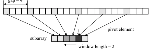
To this end, we employ the window technique [2, 3] in the Shell sort. During the insertion sort in each gap, instead of searching the position of each element in the whole partially sorted array, we search for its position in the partially sorted subarray of a certain window length, located to the left of the pivot element, as shown in Fig. 1. Fig. 1 shows an example of the modified Shell sort using the window technique, where the gap is 4 and the window length is 2. Subarrays consisting of elements that are separated by the gap are sorted using the insertion sort. To sort each subarray, it is compared only with the elements that are located to its left, within a distance equal to the window length from the pivot element to be inserted, which is called the modified Shell sort.
knowledge of the contents of elements in the arrayA[i]. Thus, Algorithm 1 can be executed in the FHE setting. In designing this algorithm, deciding the win-dow length in each gap for successfully sorting each subarray in the Shell sort for the given SFP 2−α is not a trivial problem. Along with the design of the window length for each gap, we propose a modified Shell sort with an additional parameterα. Further, the running time complexity of the modified Shell sort is determined to beO(n3/2√α+ log logn) with an SFP of 2−α. The parameterαis determined only from the SFP, regardless of the input sizen. In fact,αis consid-erably smaller thannand should be larger than or equal to√6 loge−1'2.534, the derivation of which is provided in a subsequent section of this paper. It is noted that the proposed modified Shell sort considers the trade-off between the running time complexity and the SFP.
gap = 4
subarray
window length = 2
pivot element
Fig. 1: Modified Shell sort using the window technique.
Algorithm 1: ModifiedShellSort(A[1 :n], α)
Input :An arrayA[1 :n] withnelements andα≥√6 loge−1'2.534 Output:Sorted array B[1 :n] with SFP 2−α
1 c←α+ 1 + log logn 2 p← blognc
3 for`←pto0 do 4 g←2`
5 k←min
nlq dn
2ge ·(c+`)· 1 loge
m
,l2gnmo
6 fori←2 tondo
7 u←min
n
k,di ge −1
o
8 forj ←uto1 do // swapping of A[i] and A[i−gj]
9 d1←A[i], d2←A[i−gj] 10 A[i−gj]←min{d1, d2} 11 A[i]←max{d1, d2}
12 end
13 end
3.2 Probability Distribution of Required Window Length
In this subsection, the probability distribution of required window length in each gap required for successfully sorting each subarray in the Shell sort is derived, as shown in Fig. 3. This probability distribution is essential in determining the window length of each gap in the modified Shell sort, because the properties of the tail of the probability distribution must be used to obtain the required window length.
While the analysis of the conventional Shell sort is performed for an average number of operations, the analysis of the window length in the modified Shell sort involves the maximum number of insertion operations for each subarray.
We assume that the gap sequence is powers of two, i.e., 2blognc,2blognc−1, · · · ,22,2,1. With this gap sequence, each subarray which is sorted using insertion sort has the following structure. The elements in odd positions of the subarray for a gap 2hare already sorted and the elements in even positions are also sorted for a gap 2h using the previous insertion sort for a gap 2h+1. We analyze the insertion sort under this special situation.
The array ofnelements is denoted by its index vector (a1, a2,· · ·, an), which is a permuted vector of (1,2,· · ·, n). If we handle the real data, we map each datum to its respective index in{1,2,· · ·, n}. Moreover, we assume thatnis an even integer. If nis odd, the same analysis can be applied, with an additional dummy element inserted in the rightmost position with the largest element. Several lemmas are needed for devising the main theorem of the probability distribution for the required window length.
Lemma 1. Let a = (a1, a2,· · · , a2m) be a subarray in each gap in the Shell sort with a gap sequence 2h, which is permuted from (1,2,· · · ,2m), satisfying
ai < ai+2 fori= 1,2,· · · ,2m−2. Let M(a) = max1≤i≤2m|ai−i|. Then there exists an even integerj and an odd integerk such that
M(a) =|aj−j|=|ak−k|
and(aj−j)(ak−k)≤0.
Proof. LetM1, M2, M3, andM4 be defined as
M1= max
1≤i≤m(a2i−1−(2i−1))
M2=− min
1≤i≤m(a2i−1−(2i−1))
M3= max
1≤i≤m(a2i−2i)
M4=− min
1≤i≤m(a2i−2i).
aj−j=−(ak−k). IfM1< M2,M(a) =M2=M3≥M1=M4holds, then there exist an odd indexjand an even indexk, such thatM(a) =−(aj−j) =ak−k. Thus, it is sufficient to prove thatM1=M4 andM2=M3.
To showM1 =M4 and M2=M3, we prove the following four inequalities;
M1≥M4, M1≤M4,M2≥M3, and M2≤M3.
i) Firstly, we show that M1≥M4. Consider an indexl, such thata2l−2l= min1≤i≤m(a2i−2i), which is−M4. We establish this case fora2`= 2m or
a2`<2m.
i)-1 Ifa2l= 2m,lmust bem, as 2mis the largest element. Thus, we obtain min1≤i≤m(a2i−2i) = 0 anda2i≥2ifor alli, 1≤i≤m, which implies that 1 cannot be in the even index and must be in the first index, and a1−1 = 0. Therefore, M1 = max1≤i≤m(a2i−1−(2i−1)) ≥ 0 = −min1≤i≤m(a2i−2i) =M4.
i)-2 Ifa2l<2m, we show thata2l+ 1 must be in the odd index. Leta2l+ 1 be in the even index; this implies that a2l + 1 = a2l+2, because all the elements in the even indices are already sorted. Then, we obtain
a2l+2−(2l+ 2) = (a2l+ 1)−(2l+ 2) =a2l−2l−1< a2l−2l, which is a contradiction to the assumption that a2l−2l is the minimum value, and thus,a2l+ 1 must be in the odd index. Among{1,2,· · ·, a2l−1},
l−1 elements have to be placed in the even indices in the left-side ofa2l. The remaininga2l−lelements must be placed in the odd indices in the increasing order from the first index 1. Thus, the index ofa2l+1 must be 2(a2l−l)+1. Asa2(a2l−l)+1−(2(a2l−l)+1) = (a2l+1)−(2(a2l−1)+1) =
2l −a2l, we obtain M1 = max1≤i≤m(a2i−1−(2i−1)) ≥ 2l −a2l = −min1≤i≤m(a2i−2i) =M4.
ii) We then show that M2 ≥ M3. Consider an index l, such that a2l−2l = max1≤i≤m(a2i −2i), which is M3. We establish this case for a2` = 1 or
a2`>1.
ii)-1 If a2l = 1, l must be 1, as 1 is the smallest element, and therefore, max1≤i≤m(a2i−2i) =−1. As a2i−2i ≤ −1 for all i, 1 ≤i≤m, 2m cannot belong to the even index. Thus, 2m must be in the (2m−1)-th index, anda2m−1−(2m−1) = 1. Therefore,M2=−min1≤i≤m(a2i−1− (2i−1))≥ −1 = max1≤i≤m(a2i−2i) =M3.
ii)-2 Ifa2l>1, we show thata2l−1 must be in the odd index. Leta2l−1 be in the even index. We havea2l−1 =a2l−2, because all the elements in
the even indices are already sorted. Then, we obtaina2l−2−(2l−2) = (a2l−1)−(2l−2) =a2l−2l+ 1> a2l−2l, which is a contradiction to the assumption thata2l−2lis the maximum value, and thus,a2l−1 must be in the odd index. Among{1,2,· · · , a2l−2},l−1 elements need to be placed in the even indices in the left-side of a2l. The remaining
a2l−l −1 elements have to be placed in the odd indices from the first index 1. Thus, the index of a2l−1 must be 2(a2l−l)−1. As
a2(a2l−l)−1−(2(a2l−l)−1) = (a2l−1)−(2(a2l−l)−1) = 2l−a2l, we obtain
Similarly, we can establish thatM1≤M4andM2≤M3by swapping the even indices with the odd indices. Therefore, we can prove thatM3= max1≤i≤m(a2i− 2i)≥ −min1≤i≤m(a2i−1−(2i−1)) =M2, and M4 =−min1≤i≤m(a2i−2i)≥ max1≤i≤m(a2i−1−(2i−1)) =M1. Therefore, we establish thatM1 =M4 and
M2=M3.
Lemma 2. Let a = (a1, a2,· · ·, a2m) be a subarray in the Shell sort with a gap sequence 2h, which is permuted from(1,2,· · · ,2m)satisfying a
i< ai+2 for
i= 1,2,· · ·,2m−2. LetW(a)be the required minimum window length to sort the subarray successfully. Then, we have
W(a) = max
1≤i≤2m(i−ai).
Proof. When we insertai into the partially sorted subarray, the following sce-narios can be given; ifai< i, we require a window length ofi−ai, and ifai≥i,
ai stays in place regardless of the window length.
Consider the first case, whereai< i. First, we assume thatiis even. Consider the elements to the left of ai. From the conditionai < ai+2, it is clear that all the elements in even indices to the left ofaiare less thanai. As there arei/2−1 even indices to the left ofai, the remainingai−i/2 elements in{1,2,· · ·, ai−1} have to be placed in odd indices in increasing order from the leftmost odd index. As the number of odd indices to the left ofai isi/2 andi/2> ai−i/2, all the elements less thanai are located to the left ofai.
We then assume thatiis odd. The proof is almost the same as that for the scenario in which i is even. As there are (i−1)/2 odd indices to the left ofai, the remainingai−(i+ 1)/2 elements in{1,2,· · ·, ai−1}must be placed in even indices from the first even index, in increasing order. As the number of even indices to the left ofaiis (i−1)/2 and (i−1)/2> ai−(i+ 1)/2, all the elements less than ai are located to the left ofai.
Thus, we prove that all the elements less thanaiare located to the left ofai. The partially sorted subarray, therefore, must include the elements{1,2,· · ·, ai− 1}in the indices{1,2,· · · , ai−1} in the appropriate order. This implies thatai moves to the indexai, and thus, we require a minimum window length ofi−ai. Consider the second case, in whichai≥i. It is evident thati/2≤ai−i/2, wheniis even, and (i−1)/2≤ai−(i+ 1)/2, wheniis odd. This implies that all the elements to the left ofaiare less thanai. Thus, the partially sorted subarray in the indices {1,2,· · ·, i−1} comprises elements smaller than ai. Therefore,
ai does not move to the left but stays in its position, regardless of the window length.
From Lemma 1, it is noted thatM(a) is equal toW(a).
Lemma 3. Let pk(n, m) be the number of distinct arrays (a1, a2,· · ·, am) of lengthm, whose elements from{1,2,· · · , n} are sorted in increasing order,ai<
ai+1, andmax1≤i≤m|ai−2i| ≤kis satisfied for a positive integerkandn≥m. Let (b0, b1,· · ·)and(c0, c1,· · ·)be the two arrays defined as
bi+1= (
bi+ (k+ 1) if iis even
bi+ (k+ 2) if iis odd
ci+1= (
ci+ (k+ 2) if iis even
ci+ (k+ 1) if iis odd. For2m−k≤n≤2m+k, we obtain
pk(n, m) = n
m
− X
1≤bi≤m
(−1)i+1
n
m−bi
− X
1≤ci≤m
(−1)i+1
n
m+ci
. (1)
Proof. It is clear thatpk(1,1) = 1 for allk≥1, andpk(n,1) =nforn≤k+ 2. As the element am in the last index must be 2m−k ≤ am ≤ 2m+k from max1≤i≤m|ai−2i| ≤ k, the following can be determined from the condition 2m−k≤am≤2m+k:
i) Forn <2m−k,
pk(n, m) = 0,
because the minimum possible value ofam must be 2m−k. ii) Forn >2m+k+ 1,
pk(n, m) =pk(2m+k, m),
because the maximum possible value ofammust be 2m+k. iii) For 2m−k≤n≤2m+k+ 1,
We derive the recurrence relation ofpk(n, m) using the following three cases: iii)-1 Forn= 2m+k+ 1,
It is easy to derive that
pk(2m+k+ 1, m) =pk(2m+k, m). (2)
Note that this case can be included in ii). Although this separation of the case appears unnatural, it enables us to analyzepk(n, m) well. iii)-2 For 2m−k+ 1≤n≤2m+k,
If the element in the last index m isn, the elements in the remaining indices should be selected from {1,2,· · · , n−1}, and thus, there are
pk(n−1, m−1) possible arrays. If the element in the last indexmis not
n, the elementncannot be located in one of the indices{1,2,· · ·, m−1}, because the elements are sorted in increasing order. Thus,{1,2,· · ·, n− 1} should be located in the indices{1,2,· · ·, m}, and there arepk(n− 1, m) possible arrays. Therefore, we obtain
pk(n, m) =pk(n−1, m) +pk(n−1, m−1). (3)
iii)-3 Forn= 2m−k, We obtain
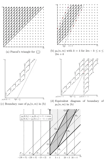
We prove the lemma using these three cases and overlapped Pascal’s triangles, as shown in Fig. 2. If we definepk(0, m) = 0 for 1≤m≤kandpk(0,0) = 1, then all of pk(n, m) are well-defined. This relation is similar to the Pascal’s triangle
n m
= nm−1
+ mn−−11
shown in Fig. 2(a), except that the width of the triangle for
pk(n, m) is limited, as shown in Fig. 2(b) as well as (2) and (4). This recursive relation can then be transformed into overlapped Pascal’s triangles. Fig. 2(c) shows a part of Fig. 2(b) near the boundary of the lower dotted line. Here, we only consider the lower dotted line. We then establish that this recursive relation near the boundary in Fig. 2(c) is equivalent to the situation of Fig. 2(d), which is two overlapped Pascal’s triangles, in whichpk(0,0) = 1 andpk(0, k+ 1) =−1. First, it can be obtained that the values on the dotted line in Fig. 2(d) are always 0, because of the symmetry of Pascal’s triangles. As adding a 0 does not change the value, the cases of Fig. 2(c) and Fig. 2(d) are equivalent corresponding to the area to the left of the dotted line.
However, the values on both the dotted lines in Fig. 2(b) must be 0. To satisfy the other boundary conditionpk(2m+k+ 2, m) = 0 on the upper dotted line in Fig. 2(b), we consider another Pascal’s triangle translated by −(k+ 2) with
pk(0,−(k+ 2)) = −1. If we add these three Pascal’s trianglesP−1, P0, and P1 shown in Fig. 2(e), there are zero boundary values on the lines from Q1 toQ2 and fromR1 toR2. However, the boundary value afterQ2 orR2is not equal to 0. To obtain the boundary values on the lines from Q2 to Q3 and from R2 to
R3, we must add the Pascal’s triangles P2 andP−2. Therefore, we repeat this
process, as shown in Fig. 2(e). The sequence{bi}in Lemma 3 is the distance from the initial vertex of P0 to that ofPi, while{ci} is the distance from the initial vertex ofP0 to that ofP−i. The initial value at the initial vertex of Pi is 1 ifi is even, and−1 ifiis odd.Qi is defined as the intersection of the boundaries of the two Pascal’s triangles starting from the initial vertices ofPi−1andP−i, and
Ri is defined as the intersection of the boundaries of the two Pascal’s triangles starting from the initial vertices ofPi andP−(i−1).
We establish that if the Pascal’s triangles Pi’s, i = · · · ,−1,0,1,· · ·, are overlapped, all of the integer points on the half-lines of −−→Q1Q2 and
−−→
R1R2 must be 0s. The integer points on the upper half-line of −−→Q1Q2 exhibit the form n= 2m+k+ 2 for all non-negative integersm, and those on the lower half-line of −−→
R1R2exhibit the formn= 2m−k−1 for allm≥k+ 1. First, in the case of the points on the half-line of−−→Q1Q2, we consider the integer points onQjQj+1, which can be denoted as n1 = 2m1+k+ 2 andbi−1 ≤m1 ≤bi. Then, we can only consider Pascal’s trianglesP−j,· · ·, Pj−1. Considering the parallel translation of
each Pascal’s triangle, the overlapped values on the points are defined as
j X
i=1 (−1)i
2m
1+k+ 2
m1+ci
+ j X
i=1
(−1)i−1 2m
1+k+ 2
m1−bi−1
. (5)
As (m1+ci) + (m1−bi−1) = 2m1+k+ 2, 2mm11+k+2+ci
= 2m1+k+2
m1−bi−1
In the case of the points on the half-line of −−→R1R2, we consider the integer points onRjRj+1, which can be denoted asn2= 2m2−k−1 andbi≤bi+1. Then, we can only consider Pascal’s trianglesPj−1,· · · , Pj. The overlapped values on the points are defined as
j X
i=1
(−1)i−1 2m
2−k−1
m1+ci−1
+ j X
i=1 (−1)i
2m
2−k−1
m1−bi
. (6)
As (m2+ci−1) + (m2−bi) = 2m2−k−1, 2mm2−k−1
1+ci−1
= 2mm2−1−kb−1
i
holds, and (6) is also equal to 0.
Therefore, we establish that with respect to the region between the two dotted lines in Fig. 2(b), Fig. 2(b) is exactly equivalent to the hashed part of Fig. 2(e). We obtainpk(n, m) by adding the values of points of several Pascal’s triangles as in (1), where the first term is from the central Pascal’s triangleP0; the second term is from the right-side Pascal’s triangles Pi’s for the positive integeri; and the third term is from the left-side Pascal’s trianglesP−i’s for the positive integer
i.
From the previous lemmas, we have the following theorem.
Theorem 4. LetC(2m, k)be the number of the permutationsaof{1,2,· · ·,2m}, such that ai< ai+2 for all possiblei, andW(a)≤k. Then, we have
C(2m, k) = 2m
m
− X
1≤bi≤m
(−1)i+1 2m
m−bi
− X
1≤ci≤m
(−1)i+1 2m
m−ci
wherebi andci are defined in Lemma 3.
Proof. As M(a) of the odd indices is equal to that of the even indices from Lemma 1, we consider only the even indices. Thus, we can consider this situation to be equivalent to the following simple situation; we consider distinctmelements from{1,2,· · · ,2m}randomly, sort them in increasing order, and considerai−2i rather than ai−i. Then,C(2m, k) is identical to pk(2m, m) in Lemma 3. This is established as m+b2m
i
= m2m−b
i
.
n
m
(a) Pascal’s triangle for mn (b)pk(n, m) with k= 4 for 2m−k≤n≤
2m+k
(c) Boundary case ofpk(n, m) in (b)
(d) Equivalent diagram of boundary of
pk(n, m) in (b)
(e)pk(n, m) using overlapped Pascal’s triangles
✁ ✂ ✁✄ ✁✄✂ ✁☎ ✁☎✂ ✁✆ ✁✆✂ ✁
✝
✄ ☎ ✆ ✝ ✂ ✞ ✟ ✠ ✡ ✄
☛
☞
✌
✍
✎
☛
☞
✌
✏
✑
✍
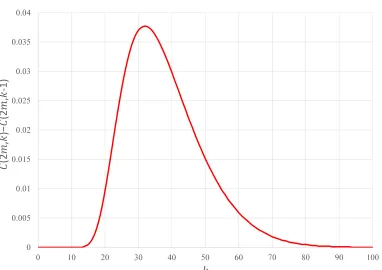
Fig. 3: Distribution ofC(2m, k)−C(2m, k−1) form= 1000.
3.3 Derivation of Running Time Complexity for a Specific SFP
In this subsection, we derive the running time complexityO(n3/2√α+ log logn) of the proposed modified Shell sort, considering the optimal trade-off with the SFP 2−α, in which α is the parameter that controls the window length of each gap. In the running time complexity, log logn increases gradually as n
increases. Therefore, the running time complexity is approximately proportional to n3/2√α. However, the probability that the output is not successfully sorted decreases exponentially asα increases. It is noted that the SFP 2−α is not re-lated to the input data size. One of the advantages of the modified Shell sort algorithm is irrespective of the size of the input data, and thus we can obtain a trade-off between the SFP and running time complexity by considering an appropriateα.
It is important to prove the following lemmas to determine the relation be-tween the binomial coefficients and exponential function. It is a well-known fact from the central limit theorem in statistics that the closer n is to infinity, the closer a binomial distribution is to a normal distribution. Even though the mial and normal distributions are similar, we should establish that some bino-mial coefficients are upper-bounded by the probability distribution function of the normal distribution. The following lemma is used in the proof of Lemma 6, and Lemma 6 is used to prove Theorem 7.
Lemma 5. Let f : [a,∞)→Rbe a function of some real number a satisfying the following;
i) lim
x→∞f(x) =M for some real number M.
ii) There exists a positive integern, such that the n-th order derivativef(n)(x) exists on(a,∞), and(−1)nf(n)(x)>0 for all x∈(a,∞).
Proof. It is sufficient to show thatf(m)(x)→0 asx→ ∞and (−1)mf(m)(x) is a monotonically decreasing function form, 1≤m≤n−1. If this is proved, then
f(x) is a monotonically decreasing function and is larger than the limit valueM
from the first condition in Lemma 5, as f0(x) is negative for (a,∞). Since it is true form=nthat (−1)mf(m)(x)>0, we will prove the following: if it is true for 2≤k≤nthat (−1)kf(k)(x)>0, then we have lim
x→∞f
(k−1)(x) = 0, and it is true that (−1)k−1f(k−1)(x) is a monotonically decreasing function.
Let gk(x) = (−1)kf(k)(x). As (−1)k−1f(k)(x) = gk0−1(x) < 0 on (a,∞),
gk−1(x) is a monotonically decreasing function. As a monotonically decreasing
function always converges to a certain value, if it possesses some lower bound, we obtain lim
x→∞gk−1(x) = T for some T, or limx→∞gk−1(x) = −∞. We assume
that lim
x→∞gk−1(x) =T for some T 6= 0, or limx→∞gk−1(x) =−∞. Then, we can
deduce someN ∈(a,∞), R >0, such that|gk−1(x)|> R, i.e.,f(k−1)(x)> Rfor allx > N, orf(k−1)(x)<−R for allx > N.
Consider the case off(k−1)(x) > R. If we integrate both terms fromN to
x∈(N,∞) iteratively as
f(k−2)(x)−f(k−2)(N) = Z x
N
f(k−1)(t)dt >
Z x
N
Rdx=R(x−N)
f(k−3)(x)−f(k−3)(N) = Z x
N
f(k−2)(t)dt >
Z x
N
R(x−N) +f(k−2)(N)dx
= R
2(x−N)
2+f(k−2)(N)(x −N),
we obtain
f(x)> R
(k−1)!(x−N) k−1+
k−2 X
i=0
f(i)(N)
i! (x−N) i,
whose right-hand side tends to infinity, as x→ ∞. In this case, f(x) tends to infinity as well, which contradicts the first condition. If we consider the case of
f(m)(x)<−R, the inequality is changed to
f(x)<− R
(k−1)!(x−N) k−1+
k−2 X
i=0
f(i)(N)
i! (x−N) i,
whose right-hand side tends to negative infinity, asx→ ∞. Thenf(x) tends to negative infinity as well, which also contradicts the first condition.
Thus, we obtain lim
x→∞gk−1(x) = 0. Asgk−1(x) is a monotonically decreasing
function,gk−1(x)>0 on (a,∞), which completes the proof.
Lemma 6. For any real numberα≥√6and any positive integern≥ dα2e, the following inequality holds
2n
n− dα√ne
< e−α2
2n
n
Proof. It can be derived that
2n n
2n n−dα√ne
=
(n+dα√ne)(n+dα√ne −1)· · ·(n+ 1)
n(n−1)· · ·(n− dα√ne+ 1) =
dα√ne−1 Y
k=0
1 + dα √
ne
n−k
.
We must prove that
dα√ne−1 Y
k=0
1 +dα √
ne
n−k
> eα2. (7)
If we consider the logarithm on the left-hand side and change the form, we obtain
dα√ne−1 X
k=0 ln
1 +dα
√
ne
n−k
≥
dα√ne−1 X
k=0
ln 1 +√ α
n−√k n
!
. (8)
Letf(x) = log 1 +αx
. Then, the right-hand side of (6) can be defined as
√
n
dα√ne
X
k=1 1 √
nf(
√
n+√1
n− k
√
n),
which is a type of Riemann sum off(x). Asf(x) is a monotonically decreasing function, the Riemann sum demonstrates its lower bound as the integration of
f(x) from√n+√1
n−
dα√√ne
n to √
n+√1
n. As √
n+√1
n−
dα√√ne
n ≤
√
n+√1
n−α, we obtain
dα√ne−1 X
k=0
ln 1 + √ α
n−√k n
! ≥√n
Z
√
n+√1 n
√
n+√1 n−
dα√√ne n
ln1 + α
x
dx
≥√n
Z
√
n+√1 n
√
n+√1 n−α
ln1 + α
x
dx. (9)
To integrate right-hand side of (9), letg(x) =xlnx. We then obtain
√
n
Z
√
n+√1 n
√
n+√1 n−α
ln1 + α
x
dx=g(n+α√n+ 1) +g(n−α√n+ 1)−2g(n+ 1).
Leth(x) = g(x2+αx+ 1) +g(x2−αx+ 1)−2g(x2+ 1) in [α,∞). If we prove lim
x→∞h(x) =α
2
, andh(3)(x)<0 in (α,∞), we obtainh(x)> α2in [α,∞) using Lemma 5. As√n≥α, we obtainh(√n)> α2, which proves (7). We must establish lim
x→∞h(x) = α
2
, andh(3)(x)<0 in (α,∞). To prove lim
x→∞h(x) =α
2 ,
we considereh(x). Usingg(x) =xlnxandh(x), we obtain
eh(x)=
1− α 2x2 (x2+ 1)2
x2−αx+1
1 + αx
x2+ 1 2αx
From lim x→∞
1 + p
x
x
=ep, we obtain lim x→∞e
h(x)=eα2
, and thus, lim
x→∞h(x) =
α2.
Moreover,h(3)(x) can be computed as
h(3)(x) =−4α
2x(x2−1){α2(x4+ 4x2+ 1)−6(x2+ 1)2} (x2+ 1)2(x2−αx+ 1)2(x2+αx+ 1)2 . Asα≥√6, we obtainh(3)(x)<0 in (α,∞). Thus, we complete the proof.
We present the following theorem, which is the main theorem of this subsec-tion.
Theorem 7. The running time complexity of the proposed modified Shell sort algorithm is obtained asO(n3/2√α+ log logn). Forα≥√6 loge−1, its SFP is upper-bounded by 2−α.
Proof. As the swapping operation in the modified Shell sort algorithm can be performed within a certain constant time, the running time complexity of the modified Shell sort in Algorithm 1 is determined from the number of swapping operations. Let S(n) be the number of the swapping operations with an input sizen. Then, S(n) can be upper-bounded as
S(n)≤n
blognc
X
`=0
k`
where the window lengthk` of each gap is defined as
r l n
2`+1 m
·(α+ 1 + log logn+`)· 1 loge
.
Thus,S(n) can be expressed as
S(n) =O
n
3 2
blognc
X
`=0 r
α+ log logn+`+ 1 2`+1
.
Using√a+b≤√a+√b, we obtain
T(n) =O
n 3 2 p
α+ log logn
blognc+1 X
`=1 1
2`2
+
blognc+1 X
`=1 √
`
2`2
.
Thus, we obtainS(n) =O(n3/2√α+ log logn), becauseP∞ `=1
1 2`2
andP∞ `=1
√
` 22`
are both finite.
that at least one subarray for the gap 2` is not successfully sorted. As B ⊆ Sblognc
`=0 B`=
Sblognc `=0
B`∩Tblognc u=`+1B
c u
, we obtain
Pr [B]≤
blognc
X
`=0 Pr
B`∩
blognc
\
u=`+1 Bcu
≤
blognc
X `=0 Pr B`
blognc
\
u=`+1 Bcu
where Tblognc u=`+1B
c
u implies the event that the sorting is successful for the gaps 2`+1,· · · ,2blognc. All of the subarrays satisfy the conditiona
i< ai+2in Theorem 4, before we perform the insertion sort for the gap 2`. Clearly, there are 2` subarrays when the gap is 2`, and the length of subarray is less than or equal to 2d n
2`+1e. Letm`=d2`n+1e, andβ`= q
(α+ 1 + log logn+`)· 1
loge. Asβ`≥ √
6,
the probability that one subarray of length 2m`is not successfully sorted can be upper-bounded as
1−C(2m`, β` √ m`) 2m` m` ≤2 2m`
m`−β` √
m`
2m`
m`
≤2e
−β2 `
where the second inequality is obtained from Lemma 6. We then obtain
blognc
X `=0 Pr B`
blognc
\
u=`+1 Bcu
≤
blognc
X
`=0
2`·2e−β2` =2
−αblognc logn ≤2
−α,
and thus, the theorem is proved.
4
Optimal Window Length by Convex Optimization
It is necessary to find the shortest window length for the SFP so that the least running time complexity of the modified Shell sort is obtained. Generally, it is not easy to derive the optimal window length in closed form. In this section, we obtain the optimal window length using convex optimization. Letβ`
p
dn/2`+1e
be the window length for the gap 2`, and Pr B`
Tblognc u=`+1B
c u
be the SFP for the
gap 2`, when sorting is successful for the gaps 2`+1,· · · ,2blognc. From Theorem
4 and Lemma 6, we obtain
Pr B`
blognc
\
u=`+1 Bcu
≤2`e−β
2 `.
The objective function that needs to be minimized is the total number of swap operations, which determines the running time. As the exact running time for-mula is rather complicated, we consider a tight upper bound of the running time, nPblognc
`=0 β` p
p` = 2`e−β
2
`. Then, we have β` = p(`+ log(1/p`))/loge. As it is sufficient to
minimizePblognc `=0
p
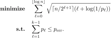
dn/2`+1e(`+ log(1/p`)), the problem of the optimal window length can be formulated as follows;
minimize
blognc
X
`=0 q
dn/2`+1e(`+ log(1/p `))
s.t. k−1 X
`=1
p`≤perr.
This formulation implies that the total running time with SFP upper-bounded
by perr needs to be minimized. We can validate that q
c+ logx1 is a convex function on small positive values, where c is a constant. As the weighted sum of convex functions is also a convex function, the objective function is a con-vex function, and the constraint is also concon-vex. Thus, this can be termed as a convex optimization problem. As every convex optimization problem can be solved using numerical analysis, it is easy to obtain the optimal window length. Then, we can deduce p`, and the optimal window length is determined to be dp
dn/2`+1e(`+ log(1/p`))/logee for each gap 2`. It is noted that the above formulation is not sufficiently tight, because it still uses the union bound. Con-structing a tighter formulation, which can be solved easily, can be a focus for future research.
5
Simulation Results
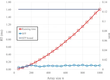
The performance of the proposed modified Shell sort is numerically verified using a personal computer with an AMD Ryzen 7 1700 CPU running at 3GHz, and 16GB RAM. First, we validate the running time and SFP when the array size varies. Then, the running time and SFP are numerically obtained when the parameter α is varied. Finally, the performance of the modified Shell sort is compared with the cases corresponding to the optimal window length, which is obtained using convex optimization, and Ciura’s optimal gap sequence, which has been validated numerically as an optimal gap sequence in non-FHE settings. The running time is mainly determined by the product of the number of swap-ping operations and the running time of the maximum or minimum function. Clearly, the running time of the maximum or minimum function is independent of the input array size orα. The relation between the performance and the main parameters of the proposed modified Shell sort is not significantly affected by the use of the homomorphic encryption scheme. Thus, in our numerical analysis, we do not use the actual homomorphic encryption scheme.
proportion ton3/2, and the SFP is independent of the array size. This numerical result coincides well with the proposed analysis of the modified Shell sort.
✁✂ ✁✄ ✁☎ ✁✆ ✁✝ ✁✝✂ ✁✝✄
✁ ✁ ✂ ✁ ✄ ✁☎ ✁✆ ✝✁ ✝✁ ✂ ✝✁ ✄ ✝✁☎ ✝✁✆
✂ ✄ ☎ ✆ ✝
✞
✟
✠
✡
☛
☞
✌
✍
✎
✏✑✑✒✓✔ ✕ ✖✗ ✘ ✙✚✚✛ ✚✜✢ ✛✣ ✤
✥✦ ✧ ✥✦ ✧★✩✙✚✪
Fig. 4: Running time and SFP of the modified Shell sort for varied array sizes.
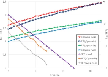
Fig. 5 shows the relation between the running time and SFP for various
α values, in which g2p denotes the power of the 2-gap sequence, gop denotes Ciura’s optimal gap sequence, and a-winand o-windenote the analytically de-rived window length and optimal window length dede-rived by convex optimization, respectively. The input array size is fixed at 1000. Similar to the previous sim-ulation, 105 input arrays are randomly generated for each αvalue. Algorithm 1 and the case corresponding to the Ciura’s optimal gap sequence or optimal window length are simulated, with the optimal window length derived using the convex optimization discussed in Section 4.
From Fig. 5, it is observed that the running time of Algorithm 1 increases as αincreases and the growth rate decreases. This observation coincides with the proposed analysis, i.e., the running time is approximately proportional to √
α. The logarithms of the SFP values of Algorithm 1 are parallel to that of the SFP bounds. This implies that the SFP is proportional to 2−α with some small proportional constant.
When the gap sequence is replaced with Ciura’s gap sequence, the running time is reduced by approximately 0.5 ms. Sorting failure is not detected in the case of the simulation that uses Ciura’s gap sequence. This implies that the order of the SFP of Ciura’s optimal gap sequence is less than or equal to 10−5. Although the window lengths of each gap in this paper are analytically derived for the power of the 2-gap sequence, a better result is obtained when Ciura’s optimal gap sequence is used. Further analyses on using Ciura’s optimal gap sequence will be included in future studies.
their values become closer asαincreases. The SFP of the case using the optimal window length for the power of the 2-gap sequence is closer to the SFP bound than that of the case using the analytically obtained window length. Thus, the running time can be reduced, while the SFP remains less than the SFP bound.
✁✂ ✁✄ ✂ ✄
✄ ✄☎✂ ✁ ✁☎✂ ✆ ✆☎✂
✝ ✞ ✁✝ ✁✞
✟
✠
✡
☛
☞
✌
✍
✎
✏
✑
✒
✓
✔
✕
✖✗✘✙ ✚✛
✜✢✣✤✥✦✧★ ✩✪✫ ✬✭ ✜✢✣✤✥✦✧✮✩✪✫ ✬✭ ✜✢✣✤✮✦✧★ ✩✪✫ ✬✭ ✜✢✣✤✮✦✧✮✩✪✫ ✬✭ ✯✰✱✲✮✳✬✴ ✯✰✱✣✤✥✦✧✮✩✪✫ ✬✭ ✯✰✱✣✤✥✦✧★✩✪✫✬✭
Fig. 5: Running time and SFP of the modified Shell sort for variedαvalues and comparison of these values with those obtained from the cases of Ciura’s optimal gap sequence and optimal window length derived by convex op-timization.
6
Conclusion and Future Work
In this paper, we proposed a modified Shell sort with a gap sequence of powers of two and an additional parameter α in the FHE setting, and derived the running time complexityO(n3/2√α+ log logn), considering a trade-off with the SFP 2−α. We also established that the running time complexity of the proposed algorithm is almost the same as the average-case running time complexity of the original Shell sort, while the SFP is maintained to be minimal. We then obtained the optimal window length of each gap by numerically solving a convex optimization problem. We believe that this study plays a significant role in the foundation of the analysis of the Shell sort in FHE settings.
We plan to use the Shell sort with other gap sequences in a future study by extending this analysis.
References
2. Chatterjee, A., Sengupta, I.: Windowing technique for lazy sorting of encrypted data. In: 2015 IEEE conference on communications and network security (CNS). pp. 633–637. IEEE (2015)
3. Chatterjee, A., SenGupta, I.: Sorting of fully homomorphic encrypted cloud data: Can partitioning be effective? IEEE Transactions on Services Computing (2017) 4. Cheon, J.H., Kim, D., Kim, D., Lee, H.H., Lee, K.: Numerical methods for
com-parison on homomorphically encrypted numbers. IACR Cryptology ePrint Archive (2019)
5. Ciura, M.: Best increments for the average case of shellsort. In: International Sym-posium on Fundamentals of Computation Theory. pp. 106–117. Springer (2001) 6. Emmadi, N., Gauravaram, P., Narumanchi, H., Syed, H.: Updates on sorting of
fully homomorphic encrypted data. In: 2015 International Conference on Cloud Computing Research and Innovation (ICCCRI). pp. 19–24. IEEE
7. Espelid, T.O.: Analysis of a shellsort algorithm. BIT Numerical Mathematics 13(4), 394–400 (1973)
8. Gentry, C.: Fully homomorphic encryption using ideal lattices. In: Stoc. vol. 9, pp. 169–178
9. Knuth, D.E.: The art of computer programming: sorting and searching, vol. 3. Pearson Education (1997)
10. Rivest, R.L., Adleman, L., Dertouzos, M.L., et al.: On data banks and privacy homomorphisms. Foundations of secure computation4(11), 169–180 (1978) 11. Shell, D.L.: A high-speed sorting procedure. Communications of the ACM2(7),