Quantitative sampling and analysis of trace elements in atmospheric aerosols: impactor characterization and Synchrotron-XRF mass calibration

www.atmos-meas-tech.net/3/1473/2010/ doi:10.5194/amt-3-1473-2010

© Author(s) 2010. CC Attribution 3.0 License.

Measurement

Techniques

Quantitative sampling and analysis of trace elements in atmospheric

aerosols: impactor characterization and Synchrotron-XRF

mass calibration

A. Richard1_{, N. Bukowiecki}1_{, P. Lienemann}2_{, M. Furger}1_{, M. Fierz}3_{, M. C. Minguill´on}4_{, B. Weideli}2_{, R. Figi}5_, U. Flechsig6, K. Appel7, A. S. H. Pr´evˆot1, and U. Baltensperger1

1_{Laboratory of Atmospheric Chemistry, Paul Scherrer Institut, Villigen, Switzerland} 2_{School of Life Sciences and Facility Management, W¨adenswil, Switzerland} 3_{University of Applied Sciences Northwestern Switzerland, Windisch, Switzerland}

4_{Institute for Environmental Assessment and Water Research (IDAEA), CSIC, Barcelona, Spain} 5_{Empa, Swiss Federal Laboratories for Materials Testing and Research, D¨ubendorf, Switzerland} 6_{Swiss Light Source, Paul Scherrer Institut, Villigen, Switzerland}

7_{Hamburger Synchrotronstrahlungslabor at Deutsches Elektronen-Synchrotron DESY, a Research Centre of the Helmholtz}

Association, Hamburg, Germany

Received: 16 April 2010 – Published in Atmos. Meas. Tech. Discuss.: 1 June 2010 Revised: 27 August 2010 – Accepted: 6 October 2010 – Published: 20 October 2010

Abstract. Identification of trace elements in ambient air can add substantial information to pollution source apportion-ment studies, although they do not contribute significantly to emissions in terms of mass. A method for quantitative size and time-resolved trace element evaluation in ambient aerosols with a rotating drum impactor and synchrotron ra-diation based X-ray fluorescence is presented. The impactor collection efficiency curves and size segregation characteris-tics were investigated in an experiment with oil and salt par-ticles. Cutoff diameters were determined through the ratio of size distributions measured with two particle sizers. Further-more, an external calibration technique to empirically link fluorescence intensities to ambient concentrations was devel-oped. Solutions of elemental standards were applied with an ink-jet printer on thin films and area concentrations were subsequently evaluated with external wet chemical methods. These customized and reusable reference standards enable quantification of different data sets analyzed under varying experimental conditions.

Correspondence to: M. Furger ([email protected])

1 Introduction

by determining the collection efficiency curves. The highly time resolved measurements of trace elements in ambient air result in low amounts of sample material in the range of a few µg per analyzed area. This demands a highly sensitive detection method such as synchrotron radiation based X-ray fluorescence spectrometry (SR-XRF), which provides a high sensitivity on small analysis areas. Bukowiecki et al. (2008) established an automated procedure to analyze many spectra in a reasonable time.

Since deviations relative to the desired size cuts would re-sult in an incorrect size attribution of the particulate mat-ter, knowledge about the size segregation characteristics of the impactor is crucial for the data quality. This paper de-scribes the determination of the inverse collection efficiency curves for the three size ranges by the use of an artificial aerosol generator. The rotating drum impactor is introduced in Sect. 2.1, followed by the results of the characterization study in Sect. 2.2. Trace elements sampled with the de-scribed impactor were analyzed with SR-XRF (see Sect. 3.1). For a quantitative analysis, raw spectral count rates have to be linked to ambient concentrations. The production of ad-equate reference standards for a consistent elemental mass calibration under different experimental conditions is the main focus of this paper, discussed in Sects. 3.2 and 3.3. Mass calibrated time resolved and size-segregated impactor data were finally compared to 24-h filter data in Sect. 4.

2 Sampling method

2.1 Impactor characterization

The rotating drum impactor (RDI; Bukowiecki et al., 2005, 2009) is a modification of the 3-stage UC Davis Rotating Drum Unit for Monitoring (3DRUM; Cahill et al., 1985). The 3DRUM was designed for continuous sampling of am-bient aerosols in three size ranges of aerodynamic diame-ter: 2.5–1.15 µm, 1.15–0.34 µm, and 0.34 to approximately 0.1 µm with a sample flow of 22.7 l min−1. The objective of the modification was to design a new impactor with step-wise rotation for a volumetric flow of 16.6 l min−1(corresponding to 1 m3h−1) and particle size segregation in ranges of 10– 2.5 µm, 2.5–1 µm, and 1 to approximately 0.1 µm. The three impactor stages will be referred to as stage 10 (PM10−2.5),

stage 2.5 (PM2.5−1) and stage 1 (PM1−0.1) in the

follow-ing. Particulate matter ≥10 µm is removed by the PM10

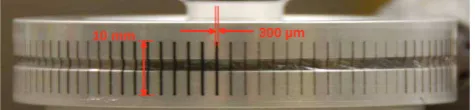
-inlet (Digitel AG, DPM10/2,3/01) on top of the instrument. Due to the stepwise movement of the drum, aerosol parti-cles are deposited in a bar-code-like structure on the film, as illustrated in Fig. 1. Modified RDI drums were designed to be used for sampling as well as for subsequent SR-XRF analysis, see Bukowiecki et al. (2008) and Sect. 3.1. These notched aluminum wheels allow the beam to pass through the wheels without interaction with metallic wheel mate-rial. They are covered with a 6-µm polypropylene (PP) film

300 µm 10 mm

Fig. 1. RDI sampling drum: a notched aluminum wheel, coated

with a 6-µm PP film, used for sampling and subsequent SR-XRF-analysis as well as for the calibration. The bar code-like structure of deposited particulate matter is visible on the film. The black color on the depicted stage 1 bars with a width of 300 µm and a height of 10 mm is mainly caused by soot deposition.

coated with Apiezon M (M & I Materials Ltd.), a silicon-free hydrocarbon grease, to reduce sampling losses due to bouncing effects. One wheel has a capacity for 96 sample bars. An advantage of the combination of RDI sampling on customized wheels with subsequent SR-XRF analysis is that measurements can take place without further sample treat-ment, unlike most conventional techniques such as induc-tively coupled plasma optical emission spectrometry (ICP-OES) and mass spectrometry (ICP-MS), reducing the risks of contamination and loss of analyte.

The impaction parameter, or Stokes number, is defined for an impactor as the ratio of the particle stopping distance at the average nozzle exit velocityUand the nozzle half-width,

Dj/2:

Stk50 =

τ U Dj/2

= ρpd

2

50U Cc(d50)

9η Dj

(1) withτ being the relaxation time,ρpthe particle density,d50

the cutoff diameter,Cc the Cunningham-slip correction

fac-tor andηthe viscosity of air. Under the assumption that the Stokes number remains the same for a given impactor design, the nozzle dimensions for the new RDI were derived through Eq. (1): first, Stokes numbers were calculated for the setup of the original 3DRUM. Based on this, the dimensions for the rectangular nozzles of the RDI with new cutoff sizes were determined accordingly as (1.52×10) mm, (0.68×10) mm and (0.3×10) mm, see Table 1 for details. Since the cut-off diameterd50 of the lowest stage of the 3DRUM is not

known precisely, it was estimated to lie in the range between 0.06 and 0.12 µm. Due to this uncertainty, thed50of the RDI

for the lowest stage is expected to lie between 0.1 and 0.2 µm. Hinds (1982) suggested an ideal Stokes number of Stk50=0.59 for 50% collection efficiency for impactors with

Table 1. Values of characteristic parameters of 3DRUM and RDI as

well as penetration midpoint diameters in µm (aerodynamic diame-ter) calculated from the second derivativeE00 dpof the sigmoidal fit for RDI stages 10, 2.5, and 1. The free parameterciof the

sig-moidal fit, which is an equivalent way to obtain the inflection point, is listed as well.

stage 10 stage 2.5 stage 1

3DRUMd50[µm] 1.1 0.34 0.06–0.12

3DRUMDj[mm] 0.82 0.31 0.25

Stk₅₀(3DRUM,RDI) 0.49 0.44 0.06–0.14

RDId50[µm] 2.5 1.0 0.1–0.2

RDIDj[mm] 1.52 0.68 0.3

dpfromE00(dp)fit 2.4±0.2 1.03±0.02 0.20±0.02

dpfromci 2.4±0.2 1.03±0.02 0.20±0.02

instrument was employed in longer field campaigns. More-over, the use of multiple small-area nozzles per impactor stage to achieve a more ideal Stokes number under low pres-sure conditions (as e.g. used in the electrical low-prespres-sure impactor – ELPI, Marjam¨aki et al., 2000) was not favorable, as the small deposition areas would add additional uncer-tainty to the applied analysis which produces the best results for large and homogeneous deposition areas. Thus, the low Stokes number for stage 1 (0.06–0.14) is a result of the con-straints of the coupled sampling and analysis method consid-ered here at the expense of a reduced impaction efficiency. 2.2 Determination of cutoff sizes

RDI characterization studies were previously conducted us-ing laboratory room air as a quasi-stable proxy for urban ambient air (Bukowiecki et al., 2009). This experimental approach was suitable for the scope of that study, but the necessary corrections through the use of room air restrict a general application. For this study, the cutoff diameters for stages 10 and 2.5 were determined through application of a condensation monodisperse aerosol generator (CMAG, TSI Inc., Model 3475), as in Kwon et al. (2003), and an aerodynamic particle sizer (APS, TSI Inc., Model 3321). Particles produced by the CMAG were quasi-monodisperse dioctyl sebacate (DEHS, C26H50O4) droplets in the size

range from approx. 0.3 to 5 µm (geometric standard devi-ation σg=1.4). Settings for the CMAG varied within the

following values: saturator flow 2.25–3 l min−1_{, saturator}

temperature 235–240◦C, while the reheater temperature re-mained constant at 100◦C. Average particle concentration produced by the CMAG was 400 particles cm−3 after a di-lution stage avoiding a too high concentration in the APS. For the cutoff determination of stage 1, particles in the order of 0.1 µm were required, which are difficult to produce with the CMAG. For this purpose, polydisperse NaCl particles

CMAG/ nebulizer APS/

SMPS

RDI RDI APS

SMPS Setup A

reference measurement

Setup B

measurements at RDI stages

APS

pump pump

10

2.5

1 10

2.5

1

CMAG/ nebulizer

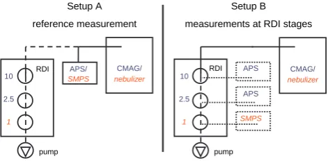
Fig. 2. Schematic layout of the two subsequent setups for cutoff

de-termination experiments: the left side illustrates the reference mea-surement (setup A), where the concentration of oil droplets pro-duced by the CMAG is measured directly with the APS. For stage 1 the NaCl concentration produced by a nebulizer is measured with the SMPS. The RDI is connected in order to simulate realistic flow conditions. The right side displays the actual experimental setup, where the APS is connected subsequently to the covers of stages 10 and 2.5 and then the SMPS is connected to the cover of stage 1 (setup B).

were produced with a nebulizer, directed through a dryer and measured with a scanning mobility particle sizer (SMPS) consisting of a differential mobility analyzer (DMA, TSI Inc., Model 3081) and a condensation particle counter (CPC, TSI Inc., Model 3025, high flow). However, higher particle bouncing is expected for NaCl particles because they do not stick as well to the substrate as the oil droplets.

While the APS is a suitable device to measure coarse parti-cles (APS size interval: 0.542–19.8 µm, aerodynamic diam-eter), the SMPS is a more adequate choice to sample par-ticles in the fine fraction (size interval of employed SMPS: 7–300 nm, mobility diameter). The mobility diameterdmob

measured with the SMPS was transformed into an aerody-namic diameterdpusing the following recursive equation:

dp = dmob q

Cc(dmob)/Cc dp pρp/ρ0 (2)

taking into account the respective Cunningham-slip-correction factorsCc dpandCc(dmob), the density of airρ0

and the density of DEHS (ρp=0.91 g cm−3) and NaCl

parti-cles (ρp=2.16 g cm−3), respectively.

1 2 3 4 5

−1.0

0.0

1.0

Aerodynamic diameter dp [µµm] E10

((

dp

))

[−]

(a) Stage 10

O data points

fit to data

E''10((dp))

0.5 1.0 1.5 2.0

−1.0

0.0

1.0

Aerodynamic diameter dp [µµm] E2.5

((

dp

))

[−]

(b) Stage 2.5

O data points

fit to data

E''2.5((dp))

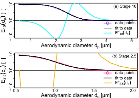
Fig. 3. Stage penetration curveEi dpfor stages 10 and 2.5: ratio of size distributions obtained in setup B versus size distributions ob-tained in setup A. The upper panel (a) shows the ratio for stage 10, a sigmoidal fit was applied to data points. The second derivative

E_i00 dpis shown on the same axis scale. The lower panel (b) shows data points and sigmoidal fit for stage 2.5,E00_2.5 dpis shown on the same axis scale.

were 5 s for each APS sample and the SMPS scanning inter-val lasted about 300 s.

Instruments were connected with conductive tubing (TSI Inc.) and attached to specially manufactured RDI stage cov-ers. Experiments were performed at ambient temperature (≈25◦C). The flow was measured with a primary flow cali-brator (A. P. Buck Inc.) and regulated with a mass flow con-troller (red-y, V¨ogtlin Ltd.) before each experiment to assure the necessary flow and pressure conditions for a correct op-eration of the RDI (i.e. 16.6 l min−1). This is especially im-portant for stage 1 because of the low cutoff diameter (0.1– 0.2 µm). Here, the jet velocity is much higher (106 m s−1 compared to 18 m s−1, stage 10, and 42 m s−1, stage 2.5) and the pressure drops from about 101 to 88 kPa. Stage 1 is close to the transition from an impaction to a diffusion con-trolled deposition regime. To ensure that identical pressure and flow conditions are maintained at the respective nozzles in both setups, inlet flow rate and pressure were monitored and adjusted accordingly. In order to accommodate for the additional flow rates when the particle sizers are connected to setup B (5 and 1 l min−1for the APS and SMPS, respec-tively), the RDI was connected also in setup A.

Size separation characteristics were obtained from collec-tion efficiency curves plotted versus aerodynamic diameter. The cutoff diameter and the stage penetration midpoint di-ameterd50both imply the diameter where 50% of particles

are collected and 50% pass through (Hinds, 1982). Inverse efficiency curvesEi dpwere computed based on the ratio

of the averaged particle size counts measured in setup B and setup A:

50 100 150 200 250

0.0

0.4

0.8

Aerodynamic diameter dp [nm]

E1

((

dp

))

[−]

(a)

O data points

fit to data

50 100 150 200 250

−4e−05

2e−05

Aerodynamic diameter dp [nm]

E''1

((

dp

))

[−]

(b)

E''1((dp))

Fig. 4. Stage penetration curveE1 dpfor stage 1: ratio of size dis-tributions obtained with the SMPS connected to the RDI (setup B) versus size distributions obtained with the SMPS connected to the nebulizer (setup A). The upper panel (a) shows the data points and the sigmoidal fit. For better readability the second derivative

E00₁ dpis displayed in the lower panel (b).

Ei dp

= countssetup Bi

countssetup A

(3)

withibeing either stages 10, 2.5 or 1. Following the concept introduced previously by Bukowiecki et al. (2009),Ei dpis

also referred to as stage penetration at a given particle sizedp,

i.e. the non-deposited particle fraction. Kwon et al. (2003) suggested a sigmoidal fit for the inverse efficiency curve:

Ei dp =

ai

1 + exp −(dp_bi−ci)

(4)

with parametersai,bi,ci, tuned to provide the best fit to the

experimental data. In this approach thed50,i are obtained

di-rectly by the parameterci, the inflection point. This is

equiv-alent to calculating the inflection point as zero point of the second derivativeE_i00 dp

. All calculated cutoff diameters are compiled in Table 1. Stage penetration curves Ei dp

and second derivativesE_i00 dpof the sigmoidal fits are

dis-played in Figs. 3 and 4. Already with little noise in the data pronounced peaks occur in the derivative, thus the concept is only applicable for the parts of the curve with very little noise. The fit in the region of diameters smaller than 100 nm for stage 1 is not as satisfactory as for the other stages be-cause variations in the size distribution in the Aitken mode (particles<100 nm) can have considerable effects on the ra-tio.

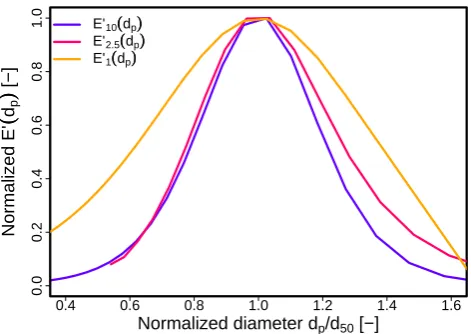
that pass through and a number of undersized particles that are collected, quantities which ideally should be symmetric. Bukowiecki et al. (2009) introduced the first derivative of

Ei dpas a measure for the cutoff sharpness, which is plotted

in Fig. 5 versus the normalized diameterdp/d50,i. For better

readability all first derivativesE0_i dpwere normalized to 1.

The curves suggest that the cutoff sharpness achieved with the tested RDI is rather broad, especially for stage 1, which was already observed by Bukowiecki et al. (2009). An impli-cation is that the size limits of individual RDI stages might be slightly smeared out and that smaller particles could be deposited on a higher stage and vice-versa. Several com-parisons to concentrations of 24-h filters obtained with high-volume samplers for PM10, PM2.5and PM1showed that this

effect is not significant on a mass base, see also Sects. 4 and Bukowiecki et al. (2005). The values derived for the cutoff diameters of stage 10 (2.4±0.2 µm) and stage 2.5 (1.03±0.02 µm) correspond well with the theoretical values 2.5 and 1.0 µm, respectively. They confirm the values ob-tained in the previous study: 2.4±0.2 µm and 1.0±0.02 µm. For stage 1 a value of 0.20±0.02 µm was found, which lies within the expected range of 0.1–0.2 µm.

Through the use of two aerosol generators, the respective aerosol concentrations were high enough to obtain cutoff di-ameters directly from the data without any further correc-tions. The presented results verify a correct size segregation within the RDI.

3 Technique for mass calibration

3.1 Synchrotron radiation based X-ray fluorescence spectrometry (SR-XRF)

The low aerosol mass on individual RDI bars demands a highly sensitive detection method. Additionally, a method for a high-throughput analysis was required for RDI sam-pling in field campaigns, where the typical number of indi-vidual samples can easily reach about 5000. SR-XRF pro-vides a sufficiently high sensitivity and easy sample han-dling, but it depends on many parameters and therefore re-quires external calibration in case not all of them are known (Rousseau et al., 1996). Calibration through model calcula-tions of mass absorption coefficients, excitation factors and instrumental characteristics (fundamental parameter analy-sis) was not applicable due to the high variability in the el-emental composition of sampled particles. Today adequate reference materials in terms of similar elemental composi-tion, particle size, sample homogeneity and substrate thick-ness for ambient aerosol analysis on PP films are still scarce. Thus a general, reusable reference, similar to the sample in terms of matrix composition and sample thickness for cal-ibration of each experimental setup and session was devel-oped to obtain a correct quantification. This provides com-parability between different analyses since conditions during

0.4 0.6 0.8 1.0 1.2 1.4 1.6

0.0

0.2

0.4

0.6

0.8

1.0

Normalized diameter dp/d50 [−]

Normalized E'

((

dp

))

[−]

E'10((dp))

E'2.5((dp))

E'1((dp))

Fig. 5. Experimental RDI cutoff sharpness: normalized first

deriva-tives ofEi dp

E0_i dp_max=1

for all RDI stages 10, 2.5 and 1

plotted versus the normalized diameter dp/d50,i. The E 0 i dp

curves represent a measure for the size-segregation sharpness in the RDI.

(h×v) wide beam irradiated the sample and a nitrogen cooled Si(Li)-detector (Sirius 80, Gresham) with a nominal resolu-tion of 144 eV (Mn Kα) measured the fluorescence counts. This detector is suitable to measure Kαlines of heavier ele-ments (up to the Ba Kαline at 32 keV) due to the large active volume (Si crystal depth: 4 mm, area: 80 mm2) and a Be win-dow thickness of 12.5 µm. Since the detection efficiency of Si(Li) detectors decreases for lighter elements as electronic noise increases, a Si drift detector with a 3-µm polymer win-dow (plus a 0.5-µm aluminum layer) and smaller active vol-ume (depth: 450 µm, area: 10 mm2) with the ability to pro-cess higher count rates was employed for measurements at the SLS. Low peaking times (in the order ofτp=1 µs) are

suitable for this detector, but would lead to a too low en-ergy resolution in the Si(Li) detector, which was operated withτp=12 µs. The efficiency of Si drift detectors decreases

rapidly for higher energies because the thin Si crystal ab-sorbs less than 30% above 11 keV. Thus, each detector is matched to the chosen excitation energies. The detector dead time was kept below 30% by reducing the size of the photon beam. Output and input count rates (OCR, ICR) were mea-sured while varying the opening of exit slits to investigate the detector saturation regime. Determining the relationship between OCR and ICR for a given detector at given experi-mental conditions enabled correcting for potential dead time effects in the detector.

Sample wheels were rotated with a goniometer in steps of 3.51◦, corresponding to the separation of individual RDI bars, and each bar was irradiated typically for 20–30 s. Since synchrotron radiation is linearly polarized, positioning the fluorescence detector in the polarization plane at an angle of 90◦ with respect to the incident beam reduced the spectral background due to coherent and incoherent scattering sub-stantially.

3.2 Absolute mass calibration

Fluorescence counts of sample elements can be linked to the area concentration (µg cm−2) if the deposited mass of one sample, chosen as reference, is determined externally by wet-chemical methods in a subsequent step. An example is ICP-OES, but it requires more analyte mass than deposited on a single RDI bar, because the sensitivity is not high enough for these minute masses. Furthermore, the sample mate-rial digestion and possible contamination error demanded a new, non-destructive method without structural modification. Since readily available calibration films of similar composi-tion and thickness as the sample do not exist, producing a customized calibration film became necessary. Fittschen et al. (2006, 2010) introduced a concept for applying picoliter droplets via an ink-jet printer on different reflector substrates for TXRF. Transforming this approach to the substrates used in SR-XRF by Bukowiecki et al. (2008) gave rise to a pro-cedure of applying standard solutions on thin films with an ink-jet printer. Calibration films were fixed on RDI sample

wheels to safeguard that experimental conditions for the SR-XRF analysis are the same.

The use of a Compact Disc-label printer (HP Photos-mart D5160), along with the film structure itself ensured op-timized adherence of the solution on the substrate because the film is not bent and transported by small brushes as in conventional printers. Clean printer cartridges (type HP 339, completely cleaned by Pelikan Ltd.) with a 15-pl ink drop volume were filled with customized solutions. A precon-dition for a correct calibration is the similarity of reference and aerosol specimen in terms of homogeneity (grain size and shape), chemical composition and concentration. This would imply using standards with a limited concentration range adapted to the concentration range of the samples. In contrast, a decreasing uncertainty of slope and intercept is obtained for more measurement points in a wider concentra-tion range (Van Grieken, 2002). Therefore, the concentraconcentra-tion range was chosen as a compromise between similarity to the sample and reduction of the uncertainty. In this range the relation between fluorescence intensity and mass per printed area is expected to behave linearly.

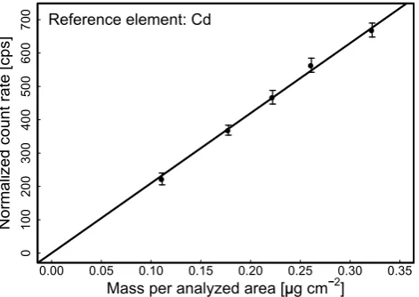
Two techniques to obtain several increasing coating densi-ties of standard solutions on the substrate were tested: print-ing one to five times the same amount of solution or printprint-ing five areas with different transparency (i.e. “color” saturation in the printer settings). Only the first technique yielded the requested linear increase in mass per coated area. For each of the five coatings pieces of 9 cm2from the same printing pro-cess were analyzed by ICP-OES. The linear relationship of fluorescence intensity (count rate normalized to photon flux and detector dead time) for the reference element Cd ver-sus the obtained mass per analyzed area ranging from 0.11 to 0.33 µg cm−2_{is plotted in Fig. 6. The slope of the fitted linear}

curve of reference element count rate (8st/tc) versus mass

per area in µg cm−2(Cst) is inserted into the calibration

for-mula introduced below (Eq. 7).

When primary X-rays interact with material, scattering and secondary fluorescence excitation occurs beside primary absorption (Giauque et al., 1979). This implies that the flu-orescence intensity of the aerosol sample is not only based on the absolute concentration but can also depend on the to-tal chemical composition (i.e. the matrix seen as sample plus substrate). Owing to the thin sample layer and low mass den-sity of collected particles, the samples are irradiated com-pletely and concentrations are too low to cause secondary X-ray absorption by lighter elements (neglecting the effects of particle size). In the investigated ambient trace element determination, matrix effects were neglected as discussed al-ready by Bukowiecki et al. (2008).

●

● ●

●

●

0.00 0.05 0.10 0.15 0.20 0.25 0.30 0.35

0

100

200

300

400

500

600

700

Mass per analyzed area [µµg cm−−2]

Normalized count rate [cps]

Reference element: Cd

Fig. 6. Fluorescence intensity of reference element Cd: individual

data points represent the average count rates (normalized to photon flux and detector dead time) for about 50 spectra of each coating on the calibration film. The absolute mass calibration factor is obtained by the slope of the linear regression (with an intercept of zero) of mean fluorescence count rates in cps versus area concentration in µg cm−2.

printing results. Commercially available films in different thickness were tested: a 100-µm ink jet transparency film (3 M, CG3420), a 100-µm PET ink jet film (Folex, BG-32.5 RS plus), both coated, a 50-µm PET film (Folex, X-131) and a 25-µm self adherent polypropylene film, both uncoated. Some films contain interfering elements like Si (adhesive of the self adherent film), S, Al, and Ca, which are also found commonly in ambient aerosol samples. Coated films contain substances for optimal homogeneous drying and the coating density increased linearly when the solution was printed sev-eral times on the same area. For the uncoated film activation in a plasma chamber before applying the solution resulted in faster drying and better adhesion to the substrate. For this purpose, an evacuated plasma chamber was filled with oxy-gen molecules ionized through a high frequency microwave. Extensive tests of different substrates, solutions and print-ing processes led to three applicable reference samples, which will be discussed in the following. First, a multi-element solution (Merck standard IV, containing Ag, Al, B, Ba, Bi, Ca, Cd, Co, Cr, Cu, Fe, Ga, In, K, Li, Mg, Mn, Na, Ni, Pb, Sr, Tl, Zn plus single elements: P, Rb, S, Sb, Se, Sn, Ti, Zr) was applied on the 100-µm PET film with a high-resolution printing process (1200 dpi). Next, a self adher-ent 25-µm PP film was tested. Again, the Merck standard solution IV was the basis and Rb and Se plasma-standards were added (10 g l−1in HNO3solution) with equal

concen-tration for each element. Through addition of 0.5% of Tri-ton X-100, a tenside to decrease surface tension, a more ho-mogenous wetting and improved drying speed was achieved. The buffered solution had a pH of 2 as a compromise be-tween the risk of corrosion of cartridges caused by a low pH

10 20 30 40

2

5

10

50

200

1000

X−ray energy [keV]

Normalized count rate [cps]

Sb

25 µµm PP film 100 µµm PET film

Fig. 7. Comparison of SR-XRF spectra of two different calibration

films: count rate of elements in the Merck IV standard solution on a 100-µm PET film and the count rate of essentially the same solution on a 25-µm PP film. Count rates measured at HASYLAB are normalized to photon flux and detector dead time.

and elemental precipitation/separation caused by a high pH. Count rates of both reference materials (on 100- and 25-µm films) are illustrated in Fig. 7, indicating a much more artic-ulated response curve for the thinner PP film due to reduced scattering. Also, the high Sb peak caused by the 100-µm PET substrate vanished for the thinner film. For measurements of the 100-µm film the beam exit slit size had to be reduced significantly to avoid saturation of the detector due to high count rates. These count rates were extrapolated according to the determined non-linear relationship between slit size and count rates due to dead time effects for the further anal-ysis. The chosen standard solution led to satisfactory results for the calibration of heavier elements.

However, to calibrate the lighter elements more precisely, a solution containing fewer elements was prepared, avoid-ing the interference of Lαlines with the Kαlines in focus. Again, clean printer cartridges were filled with a customized solution containing K, Ca and Ti standards (10 g l−1in HNO3

solution), Si (1 g l−1in HNO3/HF solution) and Al (1 g l−1in

HNO3solution). Building on the good results obtained

be-fore, this solution was applied on the self-adherent 25-µm film. The resulting calibration curve is discussed in the next section (Figs. 8 and 9). This reference led to a satisfactory result for lighter elements and showed the high potential of customized calibration solutions for specialized purposes. 3.3 Relative calibration based on external

standardization

10 20 30 40 50

0.0

0.2

0.4

0.6

0.8

1.0

Atomic number Z [−]

Efficiency [−]

Norm. count rate / count rate of Cd [−] Z0 P S Ca Cr

MnFeCo NiCu Zn

Ga Se

Rb SrZr

Cd In

fitted Srel Pabs (from Eq.6) detector effiency ω (from Eq.5)

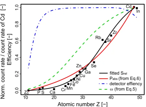
Fig. 8. Relative calibration curveSrel of Kα lines for measure-ments at HASYLAB: count rates relative to the count rates of the reference element Cd are plotted versus atomic numberZwith the corresponding fit. Theoretical curves for the fluorescence yield as calculated with Eq. (5), absorbed photon fraction as calculated with Eq. (6) (estimation for experimental conditions taking into account the HASYLAB excitation spectrum with a 8-mm Al absorber) and detector efficiency are shown on the same axis scale. The lower end of the detector efficiency is depicted byZ0in the plot, i.e. the value ofZwhere the detector efficiency reaches zero.

with increasing atomic number Z. The main reason is the Auger effect, a process competing with fluorescence in which the photon is absorbed within the atom and the re-leased energy is emitted through an Auger electron. Absorp-tion of the photon within the atom is most pronounced for lighter atoms, and significantly limits the yield of secondary X-rays from the lighter elements. The fluorescence yieldω

is the relative frequency of photon emission (in competition with the relative frequency of Auger electron emission χ; Bambynek et al., 1972; Burhop et al., 1955). An approxima-tion ofωis given by:

ω = Z 4

A+Z4 (5)

with a constant A=9×105 for the K-series and A=7×107 for the L-series. Since Auger electron and fluorescence pho-ton emission are two complementary processes, ω+χ=1. Because the calibration films (with similar substrate thick-ness and matrix compared to the samples) contain a series of elements with the same concentration, it is possible to ex-perimentally determine the response curve and calibrate the count rates with a relative factor (Srel). The empirically

deter-minedSrelcomprises all influences on the effective

fluores-cence intensity such as theoretical fluoresfluores-cence yields, mass attenuation caused by sample elements and detector sensitiv-ity. The absorbed photon fractionPabswas calculated based

on the source parameters of the DORIS III storage ring plus the 8-mm Al absorber inserted into the beam path (S´anchez

12 14 16 18 20 22

0.0

0.2

0.4

0.6

0.8

1.0

Atomic number Z [−]

Norm. count rate / count rate of Ti [−] Z0 Al Si

K Ca

Ti Srel

elements in standard solution

Fig. 9. Relative calibration curveSrelof Kαlines for measurements at SLS: count rates are normalized to detector dead time and plotted relative to the count rate of Ti, blank values are always subtracted. An exponential fit was applied to the data and shows the extrapo-lated relative calibration curveSrel for all elements in the sample. The lower end of the detector efficiency is depicted byZ₀in the plot.

del R´ıo et al., 2004) and mass attenuation coefficients of X-rays for chosen elements in the sample (Berger et al., 2007):

Pabs = X Ei< E(80)

80xs −

80

µρ

1 −e(−µρxs)

(6)

In this approximation for infinite thin films, the contributions of absorption caused by the relevant polychromatic photon intensities80for typical elements were summed up. Other

variables in the equation are the sample thicknessxs, the

to-tal absorption mass attenuation coefficient µ and the material densityρ. The calculated absorbed photon fraction reflects the overall trend of the empirical curve.

All three calculated curves were added to Fig. 8 showing the empirical relative calibration curve of Kαlines for mea-surements at HASYLAB. A sigmoidal or exponential fit to the data points turned out to provide the best extrapolation of the relative curve for those sample elements that are not contained in the calibration solution. The energy where the detector efficiency drops to zero (Z0) is included as the lower

limit of the fit. Since Cd was chosen as reference element in the absolute mass calibration, the count rates forSrelin Fig. 8

are normalized to the count rate of Cd.

Figure 9 displays the relative calibration curve Srel

Coating homogeneity, reproducibility of printed areas and stability of printed surface are challenges in the printing pro-cess. Scanning electron microscope (SEM) images from printed calibration and blank films revealed a sufficiently good homogeneity of applied droplets. The presented results show that customized calibration films for different experi-mental SR-XRF conditions can be produced with the ink-jet printer method.

3.4 Calibration formula

Spectra were fitted with the WinAxil software package (Can-berra Inc.; Van Espen et al., 1986; Vekemans et al., 2004) us-ing a least squares fittus-ing algorithm with a Bremsstrahlung background. Although the Bremsstrahlung background orig-inally has its source in the description of electron induced X-rays, where retardation of the electrons is almost com-pletely responsible for the continuum, this model was able to reconstruct the background curvature best (visual inspec-tion). Spectral counts obtained by WinAxil are calibrated with the absolute mass calibration factorCst/8stand the

rel-ative calibration factorSrel. The ambient concentrationC of

one element is deduced from the fluorescence intensity8by the following calibration formula:

C = 8 CstAi tc

8stSrelActm

1

tRDIQRDI

100 100 −td

Im

ID

(7)

with the RDI bar area (A10=15.2 mm2,A2.5=6.8 mm2 and

A1=3.0 mm2), the total calibration film area analyzed by

ICP-OES (Ac=9 cm2), the respective irradiation times for

aerosol (tm) and calibration spectra (tc), the RDI sampling

interval (tRDI), the RDI flow (QRDI), the dead time caused in

the detector (td), the actual beam current (ID) and the

maxi-mum beam current directly after injection (Im). The last term

Im/IDis only applied to measurements performed at

HASY-LAB, where the raw count rates have to be normalized to the photon flux. No correction is necessary for measurements at SLS because of a constant beam current due to top-up injec-tion. As mentioned before this calibration technique is only applicable for references with similar elemental matrix and similar film thickness.

Measurement uncertainties were calculated with uncer-tainty propagation of the three terms in Eq. (7) containing an uncertainty. The extrapolation from the rather small-sized beam spot to the RDI bar area (Abeam≈1% of total areaAi)

adds to the total measurement uncertainty with a contribu-tion of 20% of the area. Further uncertainty is introduced by possible slight variations in the RDI flow, which is esti-mated to contribute a relative uncertainty of 5%. The third term is the uncertainty obtained by the linear regression for the calculation of the absolute mass calibration factor.

Minimal detection limits (MDL) were determined as a means for the qualitative evaluation of every individual data point. Only elements exceeding the MDL with>50% of

Al Si P

S

Cl

K Ca Fe Cu Zn others

PM10-2.5

Al Si P

S _Cl

K Ca Mn Fe Zn others

PM2.5-1

Si P

S

K Fe Zn others

PM1-0.1 Mn

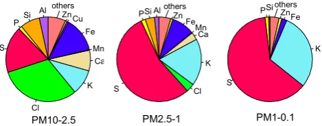
Fig. 10. Pie charts for relative contributions of measured elements

in the three size ranges (PM10−2.5, PM2.5−1and PM1−0.1) from the winter campaign in Z¨urich Kaserne obtained by RDI-SR-XRF trace element analysis.

values remained in the final data set. These detection limits are calculated as follows:

MDL = CstAi

8stSrelActRDIQRDI

3· s

8B

tm

(8)

with8Bbeing the elemental continuum counts obtained by

fitting a Bremsstrahlung background. Thus, a longer count-ing time improves the MDL for a fixed setup.

4 Discussion and selected results

The segregation into three size ranges in the RDI enables a more detailed interpretation of the relative elemental com-position. Quantitative ambient aerosol measurements can be obtained through application of the calibration for the SR-XRF method described in Sect. 3. To support and consolidate these two findings, exemplary results are presented, while the full data set will be presented in an upcoming paper. The RDI was deployed in a field campaign at Z¨urich Kaserne, Switzer-land for time and size resolved trace element sampling from 28 November 2008 to 5 January 2009 (with a short break from 26 to 28 December) and a time resolution of 2 h.

The relative elemental composition for the three size ranges is illustrated in Fig. 10. Note that for these pie charts, the period from 31 December 2008 15:00 LT to 1 Jan-uary 2009 05:00 LT is excluded to not distort the picture through unusually high emissions of some elements – e.g. S, K, Ti, Cu, Sr, Ba (and Sb) – during the fireworks at New Year’s Eve. Nonetheless, sulfur and potassium account for the highest contributions in the fine size range. Secondary sulfate and biomass combustion emissions are assumed to contribute primarily to the high sulfur concentration. Ammo-nium sulfate is formed by conversion of SO2to sulfuric acid

via either heterogeneous reactions in droplets (with ozone, NO2, H2O2) or photochemically via OH radicals (Seinfeld,

Fe contribute the highest amounts to the mass. This gain in information through the size resolution of the RDI en-hances the potential of source apportionment studies signif-icantly (Han et al., 2005; Ondov et al., 2006; Karanasiou et al., 2009).

The trace element percentage of the average PM10 mass

concentration during the campaign is obtained by the sum of PM10−2.5+ PM2.5−1+ PM1−0.1, and similarly for PM2.5.

The average mass contributed by all detected elements (Al, Si, P, S, Cl, K, Ca, Ti, Cr, Mn, Fe, Co, Ni, Cu, Zn, Sr, Zr, Mo, Cd, Sn, Sb, Ba and Pb, not extrapolated to the corre-sponding oxides) to the average PM10 mass concentration

of 24.6 µg m−3quasi-continuously monitored (every 10 min) by a tapered element oscillating microbalance (TEOM 8500) amounts to 4.6 µg m−3, thus to about 20%. The average mass concentration of PM2.5 was retrieved from daily filters of

high-volume samplers (Digitel AG, Aerosol Sampler DHA-80) to be 21 µg m−3 _{and detected elements summed up to}

3 µg m−3, corresponding to about 15% of the total PM2.5

mass concentration. Again, the period during New Year’s Eve is excluded, for more details see Table 1 in the Supple-ment.

In order to validate the obtained mass concentrations, re-sults from RDI measurements were compared to independent 24-h trace element filter data from the same campaign. Two high-volume samplers (Digitel AG, DHA-80) with PM1and

PM10 inlets were used to collect 24-h samples on 1, 3, 5, 7,

9, 11, 13, 15 and 17 December 2008. A fraction of the quartz micro-fiber filter was acid digested and subsequently ana-lyzed by ICP-OES and ICP-MS for the determination of ma-jor and minor elements (see details of the method in Querol et al., 2008). A comparison of PM10data from the filter and

the RDI analysis for characteristic elements (S, K, Fe, Cu, Sn and Sb) is shown in Fig. 11. PM1 data did not reach

the detection limit for a number of elements. Nonetheless, averaged concentrations of elements detected by both meth-ods for days of simultaneous measurements compared very well: the average concentration of PM1filter data was equal

to 0.64 µg m−3while the average concentration of PM1−0.1

RDI data summed up to 0.68 µg m−3 (this comparison in-cludes the following elements: Al, P, S, K, Ca, Ti, V, Cr, Mn, Fe, Co, Ni, Cu, Zn, Rb, Sr, Zr, Cd, Sn, Sb, Ba and Pb). Average concentrations of PM10filter data amounted to

2.7 µg m−3and the average concentration of PM10−0.1RDI

data was equal to 2.55 µg m−3, including the same elements as for PM1as well as Cl and Mo. For more details see Table 1

in the Supplement. RDI data were binned into 24-h inter-vals by calculating the mean of 12 data points, and all three RDI stages were summed up for the comparison to PM10.

Time series for the chosen elements are visualized in Fig. 11. Measurement uncertainty bars in Fig. 11 are calculated as described above for RDI data and propagated for the calcu-lation of the mean value, while the uncertainty for filter data was calculated following the method of Escrig et al. (2009). The variability of the RDI data is indicated through the 2-h

0

1000

0

1000

01. 05. 09. 13. 17. S

0

1000

0

1000

01. 05. 09. 13. 17. K filter

RDI 24h RDI 2h

0

600

1200

0

600

1200

01. 05. 09. 13. 17. Fe

0

40

0

40

01. 05. 09. 13. 17. Cu

0

4

8

0

4

8

01. 05. 09. 13. 17. Sn

Concent

ration [ng m

−

3 ]

0

4

8

0

4

8

01. 05. 09. 13. 17. Sb

Day of the month

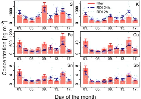
Fig. 11. Comparison of time series of 2-h RDI values to daily

high-volume filter samples. PM₁₀filter values are compared to the sum of all RDI stages from Z¨urich winter campaign for typical elements S, K, Fe, Cu, Sn and Sb. The 2-h RDI data are shown in light blue, the 12 corresponding RDI values binned to 24-h values are shown in dark blue and the 24-h filter values are shown as red bar plots. Filter samples were taken every other day on 1, 3, 5, 7, 9, 11, 13, 15 and 17 December 2008.

values in the plot, corresponding to a standard deviationσ in the order of 30–40%. Pearson correlation coefficients lie in the order of 0.9, if one outlier data point is excluded, see also Fig. 1 in the Supplement.

edges were found. For stage 2.5 a Fe particle-to-particle distance of about 30–40 µm and an overall particle-to-particle distance of less than 2 µm were estimated. These values lie within the dimensions of the beam sizes (100×200 µm and 70×140 µm).

Furthermore, TEM images were taken in that same study showing the uniformity of sampled particles on the film. The total number of particles in the coarse size range was found to be around 800 particles mm−2for a 1-h aerosol sample. The density of particles is lowest for the coarse size fraction and increasingly higher for the smaller size ranges. On the basis of this information, it is assumed that the chosen beam sizes for analysis at the SLS X05DA beam line and the HASYLAB L beam line allow for an extrapolation from the measured to total sample area if an adequate uncertainty estimate is assigned to the values. As mentioned above, the RDI bar area contributes an error of±20% to the uncertainty calculation.

In the case of the filter analysis, outliers due to sample inhomogeneity are rather improbable since the percentage of analyzed area from total sample area amounts to 12.5% (1/8 of the filter) and is thus significantly larger than for the RDI analysis. Since inhomogeneities in the distribution of the material on the filters are a function of the distance to the center, portions of the filter were taken like pieces of a round pie to avoid this influence (Brown et al., 2009).

But, since 12 RDI values are averaged to be compared to one filter value, it is difficult to find an explanation for the discrepancy in just one of the two methods. Also, correla-tions of RDI values versus filter values show no clear trend towards a general over- or under-estimation by the RDI anal-ysis and thus it is assumed that deviations lie within the un-certainties of both methods and atmospheric variability.

The gain in information obtained by a higher time reso-lution, which can lead to the identification of diurnal varia-tions, is a major advantage of the RDI method. Eventually, the overall comparison of 24-h concentration values shows reasonable agreement within the limits of both methods and therefore confirms the applicability of the presented calibra-tion methodology.

5 Conclusions

The cutoff diameters of a rotating drum impactor were mea-sured through quasi monodisperse DEHS particles and poly-disperse NaCl particles to consolidate previous studies car-ried out in laboratory room air. Results show good agree-ment with theoretical values and confirm the validity of the earlier experiment (Bukowiecki et al., 2009). However, the cutoff sharpness for the analyzed impactor is broader than that found for other cascade impactors.

The developed calibration method for SR-XRF count rates to ambient concentrations properly matched the require-ments (similar elemental composition, particle size, sam-ple homogeneity and substrate thickness for ambient aerosol

analysis on PP films) and provided an external, reusable reference material for the presented studies. The aim of obtaining consistent data sets from different experimental sessions for subsequent source apportionment studies was reached. The procedure is advantageous over already ex-isting standards as the elemental composition and the thick-ness of the substrate is comparable to the sample composi-tion and the film used for sampling. However, when using a calibration film that does not contain sufficient elements in the region of interest, adaptation to additional data, such as filter values may be necessary. Printing standard solutions on a simple transparency film with a conventional Compact Disk-label printer forms an easy to handle approach for both relative and absolute mass calibration. Averaging a series of spectra leads to a satisfactory result, although the printing ho-mogeneity might be improved in the future by using a profes-sional large-scale printer. While the substrate film thickness was appropriate in the presented case, a professional printer with the possibility to fix the film through electrostatic ad-hesion or a vacuum sample holder could lead to the use of a thinner film where lower background effects are expected.

The comparison of high time resolved and size-segregated RDI data to 24-h filter data shows generally good agreement although outliers due to the variability in both methods were observed. Despite the need for access to a synchrotron fa-cility to conduct SR-XRF analysis for high time resolution trace element data, the results demonstrate that the gain in information compared to conventional low time resolution wet-chemical evaluation justifies these efforts. High time resolution data is expected to enable a better identification of sources because daily patterns such as peak-traffic hours and other day-night differences in anthropogenic activities can be observed. This will be exploited for the current data set to perform source apportionment with positive matrix fac-torization (PMF) in an upcoming paper.

Supplementary material related to this article is available online at:

http://www.atmos-meas-tech.net/3/1473/2010/ amt-3-1473-2010-supplement.pdf.

Acknowledgements. The presented work is partly funded by the Swiss Federal Roads Office (ASTRA), the Swiss Federal Office for the Environment (BAFU) and a post-doc contract sponsored by the Spanish Ministry of Science and Innovation (MICINN). Parts of the work were performed at the Swiss Light Source, Paul Scherrer Institut, Villigen, Switzerland. We thank Andreas Jaggi for technical support at the beamline X05DA. Portions of this research were carried out at the light source facility DORIS III at HASY-LAB/DESY. DESY is a member of the Helmholtz Association (HGF). We thank Ferenc Heged¨us for his valuable input for the production of calibration standards and Marc Stammbach, Pelikan Ltd. for providing empty printer cartridges. Most of the data analysis was performed with the R software package for statistical computing (R Development Core Team , 2008).

References

Bambynek, W., Crasemann, B., Fink, R. W., Freund, H. U., Mark, H., Swift, C. D., Price, R. E., and Venugopala Rao, P.: X-ray fluorescence yields, Auger, and Coster-Kronig transition probabilities, Rev. Mod. Phys., 44, 716–813, 1972.

Berger, M. J., Hubbell, J. H., Seltzer, S. M., Chang, J., Coursey, J. S., Sukumar, R., and Zucker, D. S.: XCOM: Photon Cross Sections Database, NIST Standard Reference Database 8 (XGAM), 2007.

Berner, A. and Lurzer, C.: Mass size distributions of traffic aerosols at Vienna, J. Phys. Chem., 84, 2079–2083, 1980.

Bukowiecki, N., Hill, M., Gehrig, R., Zwicky, C. N., Liene-mann, P., Heged¨us, F., Falkenberg, G., Weingartner, E., and Baltensperger, U.: Trace metals in ambient air: hourly size-segregated mass concentrations determined by synchrotron-XRF, Environ. Sci. Technol., 39, 5754–5762, 2005.

Bukowiecki, N., Lienemann, P., Zwicky, C. N., Furger, M., Richard, A., Falkenberg, G., Rickers, K., Grolimund, D., Borca, C., Hill, M., Gehrig, R., and Baltensperger, U.: X-ray fluorescence spectrometry for high throughput analysis of at-mospheric aerosol samples: the benefits of synchrotron X-rays, Spectrochim. Acta B, 63, 929–938, 2008.

Bukowiecki, N., Richard, A., Furger, M., Weingartner, E., Aguirre, M., Huthwelker, T., Lienemann, P., Gehrig, R., and Bal-tensperger, U.: Deposition uniformity and particle size distribu-tion of ambient aerosol collected with a rotating drum impactor, Aerosol Sci. Tech., 43(9), 891–901, 2009.

Burhop, E. H. S.: Le rendement de fluorescence, J. Phys. Radium, 16, 625–629, 1955.

Brown, R. J. C., Jarvus, K. E., Disch, B. A., Goddard, S. L., and Brown, A. S.: Spatial inhomogeneity of metals in particulate matter on ambient air filters determined by LA-ICP-MS and comparison with acid digestion ICP-MS, J. Environ. Monitor., 11, 2022–2029, 2009.

Cahill, T. A., Goodart, C., Nelson, J. W., Eldred, R. A., Nasstrom, J. S., and Feeney, P. J.: Design and evaluation of the DRUM impactor, Particulate Science and Technology, Hemi-sphere Publications, Washington, DC, Proceedings of Inter-national Symposium on Particulate and Multiphase Processes, 1985.

Cliff, S. S., Cahill, T. A., Jimenez-Cruz, M., and Perry, K. D.: Syn-chrotron X-Ray fluorescence analysis of atmospheric aerosols using ALS beamline 10.3.1: application to atmospheric pollu-tion evolupollu-tion and transport, Abstr. Pap. Am. Chem. S., 225, 837, 2003.

D’Alessandro, A., Lucarelli, F., Mando, P. A., Marcazzan, G., Nava, S., Prati, P., Valli, G., Vecchi, R., and Zucchiatti, A.: Hourly elemental composition and sources identification of fine and coarse PM₁₀ particulate matter in four Italian towns, J. Aerosol Sci., 34, 243–259, 2003.

Escrig, A., Monfort, E., Celades, I., Querol, X., Amato, F., Min-guill´on, M. C., and Hopke, P. K.: Application of optimally scaled target factor analysis for assessing source contribution of ambi-ent PM10, J. Air Waste Manage., 59(11), 1296–1307, 2009. Fittschen, U., Hauschild, S., Amberger, M. A., Lammel, G.,

Streli, C., F¨orster, S., Wobrauschek, P., Jokubonis, C., Pep-poni, G., Falkenberg, G., and Broekaert, J. A. C.: A new tech-nique for the deposition of standard solutions in total reflection X-ray fluorescence spectrometry (TXRF) using pico-droplets

generated by inkjet printers and its applicability for aerosol anal-ysis with SR-TXRF, Spectrochim. Acta B, 61, 1098–1104, 2006. Fittschen, U. and Havrilla, G. J.: Picoliter droplet deposition using a prototype picoliter pipette: control parameters and application in micro X-ray fluorescence, Anal. Chem., 82, 297–306, 2010. Flechsig, U., Jaggi, A., Spielmann, S., Padmore, H. A., and

Mac-Dowell, A. A.: The optics beamline at the Swiss Light Source, Nucl. Instrum. Meth. A, 609, 281–285, 2009.

Giauque, R., Garrett, R. B., and Goda, L. Y.: Determination of trace elements in light element matrices by X-ray fluorescence spec-trometry with incoherent scattered radiation as an internal stan-dard, Anal. Chem., 51, 511–516, 1979.

Han, J. S., Moon, K. J., Ryu, S. Y., Kim, Y. J., and Perry, K. D.: Source estimation of anthropogenic aerosols collected by a DRUM sampler during spring of 2002 at Gosan, Korea, At-mos. Environ., 39, 3113–3125, 2005.

Hering, S. V. and Friedlander, S. K.: Design and evaluation of a new low-pressure impactor, Environ. Sci. Technol., 13, 184– 188, 1979.

Hinds, C. W.: Aerosol Technology, Properties, Behavior, and Mea-surement of Airborne Particles, John Wiley and Sons, New York, 1982.

Karanasiou, A. A., Siskos, P. A., and Eleftheriadis, K.: Assessment of source apportionment by positive matrix factorization analysis on fine and coarse urban aerosol size fractions, Atmos. Environ., 43, 3385–3395, 2009.

Kwon, S. B., Lim, K. S., Jung, J. S., Bae, G. N., and Lee, K. W.: Design and calibration of a 5-stage cascade impactor (K-JIST Cascade Impactor), J. Aerosol Sci., 34, 289–300, 2003. Lundgren, D.: An aerosol sampler for determination of particulate

concentration as a function of size and time, JAPCA J. Air Waste Ma., 17, 225–229, 1967.

Marjam¨aki, M., Keskinen, J., Chen, D.-R., and Pui, D. Y. H.: Perfor-mance evaluation of the electrical low-pressure impactor (ELPI), J. Aerosol Sci., 31(2), 249–261, 2000.

Marple, V., Rubow, K. L., and Behm, S. M.: A microorifice uni-form deposit impactor (MOUDI): description, calibration, and use, Aerosol Sci. Tech., 14, 434–446, 1991.

Marple, V.: History of impactors – the first 110 years, Aerosol Sci. Tech., 38, 247–292, 2004.

Ondov, J. M., Buckley, T. J., Hopke, P. K., Ogulei, D., Par-lange, M. B., Rogge, W. F., Squibb, K. S., Johnston, M. V., and Wexler, A. S.: Baltimore Supersite: highly time- and size-resolved concentrations of urban PM_2.5and its constituents for resolution of sources and immune responses, Atmos. Environ., 40, 224–237, 2006.

Querol, X., Pey, J., Minguill´on, M. C., P´erez, N., Alastuey, A., Viana, M., Moreno, T., Bernab´e, R. M., Blanco, S., C´ardenas, B., Vega, E., Sosa, G., Escalona, S., Ruiz, H., and Art´ı˜nano, B.: PM speciation and sources in Mexico during the MILAGRO-2006 Campaign, Atmos. Chem. Phys., 8, 111–128, doi:10.5194/acp-8-111-2008, 2008.

R Development Core Team: R: A language and environment for statistical computing. R Foundation for Statistical Computing, http://www.R-project.org, last access: 15 May 2010, Vienna, Austria, ISBN 3-900051-07-0, 2008.

Rousseau, R., Willis, J. P., and Duncan, A. R.: Practical XRF cal-ibration procedures for major and trace elements, X-ray Spec-trom., 25, 179–189, 1996.

S´anchez del R´ıo, M. and Dejus, R. J.: XOP 2.1: a new version of the X-ray optics software toolkit, in: Synchrotron Radiation In-strumentation: Eighth International Conference, edited by: War-wick, T., Arthur, J., Padmore, H. A., and Stohr, J., American Institute of Physics, 784–787, 2004.

Seinfeld, J. H. and Pandis, S. N.: Atmospheric Chemistry and Physics: From Air Pollution to Climate Change, John Wiley and Sons, New York, 1998.

Vekemans, B., Vincze, L., Brenker, F. E., and Adams, F.: Process-ing of three-dimensional microscopic X-ray fluorescence data, J. Anal. Atom. Spectrom., 19, 1302–1308, 2004.

Van Espen, P., Janssens, K., and Nobels, J.: AXIL-PC, software for the analysis of complex X-ray spectra, Chemometr. Intell. Lab., 1, 109–114, 1986.