An automatic contrail tracking algorithm

(1)

Atmos. Meas. Tech., 3, 1089–1101, 2010 www.atmos-meas-tech.net/3/1089/2010/ doi:10.5194/amt-3-1089-2010

Atmospheric

Measurement

Techniques

An automatic contrail tracking algorithm

M. Vazquez-Navarro, H. Mannstein, and B. Mayer

Deutsches Zentrum für Luft- und Raumfahrt, Institut für Physik der Atmosphäre, Oberpfaffenhofen, Germany Received: 16 March 2010 – Published in Atmos. Meas. Tech. Discuss.: 1 April 2010

Revised: 16 July 2010 – Accepted: 16 July 2010 – Published: 19 August 2010

Abstract. A method designed to track the life cycle of contrail-cirrus using satellite data with high temporal and spatial resolution, from its formation to the final dissolution of the aviation-induced cirrus cloud is presented. The method follows the evolution of contrails from their linear stage until they are undistinguishable from natural cirrus clouds. There-fore, the study of the effect of aircraft-induced clouds in the atmosphere is no longer restricted to linear contrails and can include contrail-cirrus. The method takes advantage of the high spatial resolution of polar orbiting satellites and the high temporal resolution of geostationary satellites to identify the pixels that belong to an aviation induced cloud. The high spa-tial resolution data of the MODIS sensor is used for contrail detection, and the high temporal resolution of the SEVIRI sensor in the Rapid Scan mode is used for contrail tracking. An example is included in which the method is applied to the study of a long lived contrail over the bay of Biscay.

1 Introduction

Contrails are ice clouds and their radiative effects are sim-ilar to that of thin cirrus clouds (Fu and Liou, 1993). The presence of aircraft induced cloudiness, contrail-cirrus, can modify the radiative properties of the atmosphere and there-fore influence the climate system. The aim of this work is to provide a tool to distinguish between natural and anthro-pogenic clouds by studying the life cycle of contrails.

The detection of cirrus contrails over areas with high air traffic density will provide a better knowledge of the cover-age and radiative forcing of man-made cirrus clouds. The current knowledge about this type of clouds is still poor (Lee

Correspondence to: M. Vazquez-Navarro ([email protected])

et al., 2009). Moreover, a time series from high resolution satellite data would be useful for studies examining changes in cirrus cloudiness in relation to air traffic over Europe and the North Atlantic such as Zerefos et al. (2003); Schumann (2005)

In satellite images, young contrails can be easily identified thanks to their linear shape. Linear contrail coverage as re-ported by Bakan et al. (1994) and Mannstein et al. (1999) has been the main source of information for the model studies on the global effect of air traffic on the radiative forcing (Ponater et al., 2002). If the atmosphere presents the necessary condi-tions, contrails can evolve into contrail-cirrus, which spread and lose their characteristic linear shape. Thus, in a single satellite image they cannot be distinguished from natural cir-rus clouds. This paper describes an automatic method that fulfils this gap. The method follows the development of a contrail from its linear stage to identify a contrail cirrus as such. Therefore, a larger number of aircraft induced clouds, not only linear contrails can be identified and studied. This will provide a more robust knowledge of their influence in climate, until now restricted to case studies.

(2)

1090 M. Vazquez-Navarro et al.: ACTA

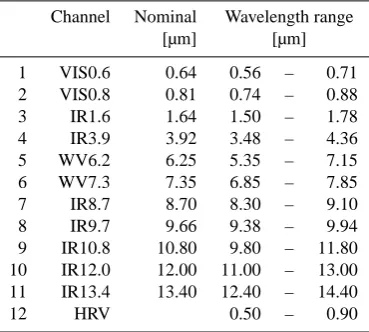
Table 1. MSG/SEVIRI spectral channels.

Channel Nominal Wavelength range

[µm] [µm]

1 VIS0.6 0.64 0.56 – 0.71 2 VIS0.8 0.81 0.74 – 0.88 3 IR1.6 1.64 1.50 – 1.78 4 IR3.9 3.92 3.48 – 4.36 5 WV6.2 6.25 5.35 – 7.15 6 WV7.3 7.35 6.85 – 7.85 7 IR8.7 8.70 8.30 – 9.10 8 IR9.7 9.66 9.38 – 9.94 9 IR10.8 10.80 9.80 – 11.80 10 IR12.0 12.00 11.00 – 13.00 11 IR13.4 13.40 12.40 – 14.40

12 HRV 0.50 – 0.90

as much as possible because the tracking algorithm consid-ers all inputs are indeed contrails. Therefore, the geometrical thresholds used in CDA this work are: a minimum length threshold (47 MODIS pixels), a minimum number of pix-els threshold (19 pixpix-els) and an alignment threshold (corre-lation coefficient>0.975). As the length threshold is larger than the number of pixels threshold, the contrail may be a non-connected structure. The physical thresholds are scene-dependent, and are related to the sum of the normalised im-ages, to the brightness temperature difference and to the gra-dient of the temperature in channel 12 µm (Mannstein et al., 1999). The CDA has already been used to retrieve the cover-age by linear contrails for several regions of the Earth: Cen-tral Europe (Meyer et al., 2002), North America (Palikonda et al., 2005), Eastern North Pacific (Minnis et al., 2005) and Southern and Eastern Asia (Meyer et al., 2007).

Data with high spatial and temporal resolution are nec-essary to locate the contrails and to track them throughout their lifetime. Given the high variability of the life cycle of contrails, it is essential to develop an algorithm that can track them in all possible situations. To study the largest amount of contrails possible, data covering heavily flown re-gions of the Earth such as the North Atlantic flight corridor and Europe are necessary. Radiometers fulfilling these re-quirements are the MODerate-resolution Imaging Spectrora-diometer (MODIS), on board of Terra (flagship of NASA’s Earth Observation System) and the Spinning Enhanced Visi-ble and Infrared Imager (SEVIRI), on board of the Meteosat Second Generation (MSG) satellites.

Terra’s orbit is near-polar and sun-synchronous, descend-ing across the Equator at 10:30 a.m., with a repeat cycle of 16 days. Terra orbits at an altitude of 705 km and, thus, the spatial resolution of its instruments is better than that of geo-stationary satellites at 36 000 km height. MODIS is a 36-band radiometer that provides measurements of the Earth with very high spatial resolution. Here, MODIS radiances

M. Vazquez-Navarro et al.: ACTA 13

Fig. 01. Four examples of BTD images showing the evolution of

contrails over southern Sweden over three hours. 06:30 UTC: con-trails appear as linear structures with a high BTD signal (light grey – white). It can be seen that the older contrails are, the more diffi-cult is to identify them as such without temporal information. Date: 3 July 2009.

Fig. 1. Four examples of BTD images showing the evolution of contrails over southern Sweden over three hours. 06:30 UTC: con-trails appear as linear structures with a high BTD signal (light grey – white). It can be seen that the older contrails are, the more diffi-cult is to identify them as such without temporal information. Date: 3 July 2009.

with a spatial resolution of 1 km are used to identify the posi-tion of the linear contrail and provide an input to the tracking algorithm.

SEVIRI is a geostationary instrument which measures ra-diances in 12 different spectral channels (see Table 1). Its sampling frequency (15 min) enables monitoring of rapidly evolving events such as contrails. The Rapid Scan Service (RSS) from MSG-1 (Meteosat-8), which provides data every 5 min started mid-2008 from a position at 9.5◦E. The region covered by the rapid scan service ranges from approximately 15◦N to 70◦N covering Europe, Northern Africa and part of the North Atlantic. These rapid scans are extremely useful for the study of the evolution of contrails.

2 Automatic Contrail Tracking Algorithm

(3)

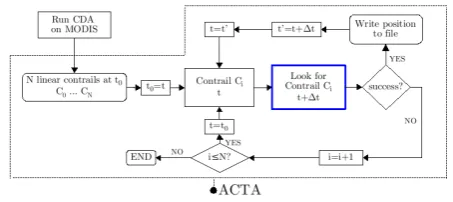
Fig. 02. Schematic representation of ACTA. Input: list of linear contrails detected by the CDA on MODIS.

Fig. 2. Schematic representation of ACTA. Input: list of linear con-trails detected by the CDA on MODIS.

a strong BTD signal to the sensor and lying close to the po-sition of that contrail in the previous image. The tracking of a contrail is a complex task because contrails change in position and shape between two consecutive satellite images. SEVIRI rapid-scan data have been used in this work because, within a 5-min time lapse, neither the shape nor the position of the contrail present major changes.

Figure 2 shows a schematic outline of ACTA. Running CDA on a MODIS image provides a list of N linear con-trails at time t0 as input to ACTA. This input contains the geographical position of the two end points of each linear contrail detected by the CDA. The latitude and longitude of both ends are used to map the contrail on the SEVIRI grid, making a parallax correction assuming a height of 10 km for the contrail. Based on the position of the contrailCiat timet,

Ci(t ), ACTA looks forCi in the following SEVIRI image, at

timet+1t,Ci(t+1t ). If it is found, then ACTA uses the

in-formation about the new position to iterate the process, with t+1t as initial time. Once the contrail cannot be tracked any longer, ACTA proceeds to the next contrail on the input list.

A very important feature of ACTA is that it is applied for-wards and backfor-wards in time. The algorithm takes the first input from CDA at timet0, the time of the MODIS overpass, and then tracks each contrail with positive or negative time increments (1t), i.e. it tracks equally back to the past and forth to the future. Thus, the contrail lifetime can be deter-mined, from its first detection in satellite at time t0−n1t until it can no longer be discriminated from its surroundings by the satellite att0+n01t, regardless of the MODIS over-pass time.

To perform the tracking, ACTA uses the brightness temperature difference (BTD) between channels IR 108 (10.8 µm) and IR 120 (12.0 µm) of SEVIRI. As it can be seen in Fig. 1, contrails are easier to identify in those im-ages because they have a larger BTD than the surroundings. This channel combination has long been used to identify thin clouds, especially thin cirrus. Ice crystals behave differently in those two wavelengths while other atmospheric and sur-face properties are similar for both channels (Lee, 1989). The

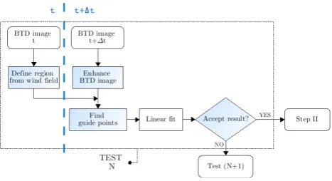
Fig. 03. Schematic overview of ACTA. Input for Step I is the MODIS detected contrail att. After Step I,mandb, the coordinates of a y=mx+bline are used as input for Step II. Output of Step II are the pixels that belong to the contrail atFig. 3. Schematic overview of ACTA. Input for Step I is the MODISt+ ∆t.

detected contrail att. After Step I,mandb, the coordinates of a

y=mx+bline are used as input for Step II. Output of Step II are the pixels that belong to the contrail att+1t.

exclusive use of infrared channels in the design enables the algorithm to run indistinctly on day and nighttime scenes.

Briefly, the process of finding the contrailCi(t+1t )(in

blue in Fig. 2) consists of two steps (see detailed flowchart in Fig. 3 and a more detailed explanation in the following pages):

(4)

Fig. 04.Schematic representation of a test in Step I. Inputs: Contrail position in the BTD image attand BTD image att+ ∆t. Each shaded box has diferent internal thresholds/definitions in each test. The output (input for Step II) is the position of the line att+ ∆t.

Fig. 4. Schematic representation of a test in Step I. Inputs: Contrail position in the BTD image att and BTD image att+1t. Each shaded box has diferent internal thresholds/definitions in each test. The output (input for Step II) is the position of the line att+1t.

– In Step II, ACTA’s task is to establish the contrail shape att+1t. ACTA uses the information of the position of the line at timet+1t (Step I) as input to define a region in which to search for the rest of the pixels that also belong to the contrail. Through a combination of image processing techniques and BTD information, the pixels belonging to the contrail are retrieved. The output of Step II, and therefore of ACTA, is at least one group of at least three connected pixels. Depending on the latitude and longitude, a connected region of 3 pixels in the area under study corresponds to an area of 50– 200 km2.

After both steps are successfully performed, ACTA writes the output (the contrail pixels) to a file and proceeds to the following iteration (i.e. the new start time ist+1t) using as start and end points the position of the westernmost and the easternmost pixels detected in Step II. If no new line param-eters are found, the tracking stops.

2.1 Step I: contrail position

In ACTA, a contrail is essentially a group of pixels with a stronger BTD signal than the surroundings, similar to a cirrus cloud but with a distinct evolution pattern. When the contrail is young, those pixels are strongly aligned. The group may change shape as it ages, but it will always retain part of its former linear shape. Therefore, a contrail can be tracked by locating that linear part throughout its lifetime. LetC(t )be the contrail att andC(t+1t )the same contrail att+1t. AsC(t )andC(t+1t )are the same contrail, the slope and intercept of the line that corresponds toC(t+1t )through the fit of the guide points will be related to the slope and intercept of the line that corresponds to contrailC(t ). To establish the parameters of the line that corresponds to contrailC(t+1t ) from the parameters of the line that corresponds to contrail C(t ), Step I performs a set of five consecutive tests. Each

M. Vazquez-Navarro et al.: ACTA

17 Fig. 05.

Annual mean (2007) zonal (top) and meridional

(bot-tom) components of the wind field at approximately 10 km height.

Source: ECMWF (European Centre for Medium-Range Weather

Forecasts).

M. Vazquez-Navarro et al.: ACTA

17 Fig. 05.

Annual mean (2007) zonal (top) and meridional

(bot-tom) components of the wind field at approximately 10 km height.

Source: ECMWF (European Centre for Medium-Range Weather

Forecasts).

Fig. 5. Annual mean (2007) zonal (top) and meridional (bot-tom) components of the wind field at approximately 10 km height. Source: ECMWF (European Centre for Medium-Range Weather Forecasts).

test has the same structure but different internal variables, and is designed to take into account various atmospheric and surface conditions. Figure 4 shows a short flowchart of a test in Step I, the shaded boxes represent the different internal variables of the tests.

The sequence of the tests is designed to identify contrails in images of increasing difficulty. Isolated contrails are easier to track than contrails surrounded by other cirrus clouds or contrails nearby. Moreover, the younger the contrail is, the more linear its shape appears in the BTD image and the easier the tracking is.

Next, a thorough definition of the internal test variables is given. Then, their thresholds and combination in each of the tests is explained. Finally, an example is shown where all five tests have been used.

Wind field-defined region1

First, to find C(t+1t ) from the information provided by C(t ), ACTA selects a region, Bij, where C(t+1t ) could

1_{Throughout the section, A}

ij or A(i,j ) denote matrices of

Ni×Nj elements. Multiplication (·) does not imply matrix

(5)

(a) (b) (c)

(d) (e) (f)

Fig. 06.Test 3.(a)Scene at timetwith contrailC(t)in the centre of the image.(b)Same scene at timet0=t+ ∆t, contrailC(t0)in the centre of the image between the white lines that delimit the area whereCcan lie after being drifted by the wind.(c)Enhanced BTD image.

(d)Selected wind field related region over the enhanced image.(e)Guide points.(f)Linear fit.

Fig. 6. Test 3. (a) Scene at timetwith contrailC(t )in the centre of the image. (b) Same scene at timet0=t+1t, contrailC(t0)in the centre of the image between the white lines that delimit the area whereCcan lie after being drifted by the wind. (c) Enhanced BTD image. (d) Selected wind field related region over the enhanced image. (e) Guide points. (f) Linear fit.

exist. This region must be consistent with the wind field at the contrail height (see Fig. 5). At a typical altitude of 10 km, and with a1t of 5 min, the wind drifts the contrail ap-proximately 10 km from its original position (depending on the speed of the wind and on the latitude and longitude, this corresponds to 2 or 3 pixels). Moreover, the wind field at flight-level height is mainly West-East, so the contrail will be most likely drifted eastwards in the region under study. These assumptions are enough for the tracking and no addi-tional wind-field data will be used.

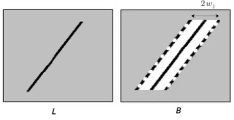
To establish the allowed region at timet+1t, ACTA fo-cuses on the line that corresponds to the contrail at time t (y=mx+b). The length of the line is limited by x=i0 andx=i1. In the first iteration,i0andi1are given by the western- and easternmost points of the contrail±10 pixels. These loose boundary conditions allow the contrail to grow and adjust its length, in case the CDA has not provided the full length of the contrail. In further iterations,i0andi1are issued from the output of Step II. The line is placed on a 2-dimensional array Lij of the same size as the BTD image

(see Fig. 7, left):

Lij=

  

 

1 ,∀(i,j ) | j=f (mi+b) ,i0< i < i1

0 , otherwise

(1) where f (x)=round(x)= bx+0.5c =max{n∈_Z|n≤x}

roundsxto the nearest integer.

Then, the region of width 2w1 (test-dependent, see Ta-ble 2) where the contrail can move from its position at timet

Fig. 07.Left: 2-dimensional arrayLwith the line corresponding to contrailC. Right: 2-dimensional arrayBwith the area (white) in which contrailC(t+ ∆t)is expected to be found.

Fig. 7. Left: 2-dimensional arrayLwith the line corresponding to contrailC. Right: 2-dimensional arrayBwith the area (white) in which contrailC(t+1t )is expected to be found.

to its new position att+1t, can be defined by shifting Lw1 pixels eastwards andw1pixels westwards (see Fig. 7, right).

Bij=

2w1

X

k=0

L(i−w1+k,j ) ,∀(i,j ) (2)

Enhanced BTD image

To enhance the contrail structures and eliminate most of the background information, ACTA applies a high-pass filter to the BTD image. First, the BTD image att+1tis smoothed using a boxcar filter. Let BTDij be the BTD image, and let

(6)

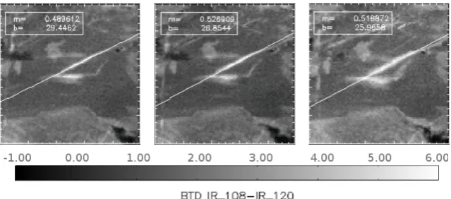
Fig. 08. Output of Step I: Contrail with its corresponding line at different stages of its development. On each plot, the liney=mx+b equation parameters. Left: at timet. Centre: at timet+25 min. Right: at timet+55 min. Background: BTD image 10.8 µm–12.0 µm, in K.

Fig. 8. Output of Step I: Contrail with its corresponding line at different stages of its development. On each plot, the liney=mx+bequation parameters. Left: at timet. Centre: at timet+25 min. Right: at timet+55 min. Background: BTD image 10.8 µm–12.0 µm, in K.

Table 2. Description of ACTA’s Step I tests.aScene-dependent cri-terion, see explanation in text below (description of Test 5).bO: ori-entation, A: alignment.

Test Region Filter Guide points Linear regression

w1 width threshold acceptance

w2 CRIT criterion(b)

1 5 pixels 2 pixels 1 K O

2 5 pixels 10 pixels 1.3 K A

3 2 pixels 2 pixels 1 K O

4 2 pixels 6 pixels 1 K A and O

5 2 pixels 10 pixels a A

The filtered image, Fij, then equals:

Fij=

          

         

1 2w2

w2−1

X

p=0

w2−1

X

q=0

BTD(i−w2

2 +p,j− w2

2 +q) , fori=(w2−1)

2 ,...,Ni−

(w2+1)

2 j=(w2−1)

2 ,...,Nj−

(w2+1)

2

BTDij , otherwise

(3) Finally, ACTA uses this information to produce an enhanced image, BTDij−Fij, and focuses on the allowed region by

multiplying by Bij (see Eq. 2).

Sij=Bij·(BTDij−Fij) (4)

The matrix Sijnow contains the enhanced BTD values in the

region shown in white in Fig. 7, right, and otherwise, 0.

Guide points

ACTA looks in Sij for the pixels that provide a stronger

sig-nal. Those points are called guide points, (i,j )0...(i,j )n,

and fulfil an empirically derived threshold, CRIT (a test-dependent scalar, see Table 2):

guide points= {(i,j ) | Sij>CRIT}, (5) Acceptance criterion

If there are less than three guide points, ACTA stops the cur-rent test and proceeds to the following test. If three or more guide points are present, a linear regression is performed and a final criterion, acceptance criterion, must be fulfilled. The acceptance criterion is test-dependent (see Table 2) and spec-ifies empirically defined requirements regarding either the correlation coefficient issued from the fit,R, (alignment cri-terion), or the orientation of the line with respect to the for-mer orientation at timet (orientation criterion), or both. If the linear regression fulfils the requirements, the position of the line issued from this regression is written to a file and will be used as input for the next iteration. Otherwise, ACTA proceeds to the following test.

The orientation criterion means that the orientation of the line that guide points define must not differ by more than 2.8◦ from the orientation of the line in the previous timestep. The alignment criterion means that the correlation coefficient of the fit through the guide points must be larger than 0.98.

(7)

M. Vazquez-Navarro et al.: ACTA 1095 empirically. They are summarised in Table 2 and explained

in detail in the following pages. If all tests provide a negative answer, the tracking stops.

Typically, Step I ends successfully already after the first or second test, depending on the image. These tests are de-signed to identify easily recognisable contrails, narrow struc-tures with a strong BTD signal. Besides, the region defined in Tests 1 and 2 is wide enough to allow the tracking of the contrail even if the wind field is particularly strong and drifts the contrail far away. When the scene is too complex be-cause of neighbouring contrails or other surrounding clouds crossing the tracked one, Tests 1 and 2 do not provide con-clusive results because they focus on a large region that may include structures other than the desired contrail. Therefore, ACTA looks for the contrail in narrower regions, such as in the Tests 3 and 4. These tests are designed for complicated cases and prevent other clouds’ pixels from being selected as contrail pixels. In particular, they impose strong require-ments on the width of the wind field-defined region and on the acceptance criterion for the line parameters. The pres-ence of alien pixels would modify too much the orientation of the contrail. Finally, ACTA’s Test 5 is usually applied to scenes with poor contrast, typically when a vanishing con-trail must be distinguished from the (similar) background.

Test 1

The first of the five tests uses a narrow smoothing filter pro-viding an only slightly smoothed BTD image att0=t+1t. The wind field-related region defined by the contrail att is wide enough so that the whole contrailC(t0)lies in it. The acceptance criterion for the line is based on the comparison of the orientation of the new line (att0) with the orientation of the line att. Due to the nature of the wind field, the ori-entation criterion ensures that the line identified corresponds to the desired contrail and not to a different contrail crossing the scene or to other natural structures present att0.

w1= 5 pixels,w2= 2 pixels, CRIT>1 K, Acceptance criterion:

m−0.05< m0< m+0.05 (orientation within 2.8◦)

Test 2

If Test 1 does not succeed, a second test is performed. Within the same pixel neighbourhood as in the prior test, a stronger filter is applied. Therefore, only the more relevant pixels are retained. In this case, the acceptance criterion of the linear fit is the alignment of the guide points (correlation coefficient).

w1= 5 pixels,w2= 10 pixels, CRIT>1.3 K, Acceptance criterion:R >0.98

Test 3

The third test is similar to the first one but constrains the exis-tence of the contrailC(t0=t+1t )to a narrower

neighbour-hood to reduce the possibility that the contrail guide points have been misidentified or outnumbered by strong BTD sig-nals from surrounding cloudiness in the prior tests. Accord-ing to the typical wind speed at 10 km height, the contrail C(t0)must lie within this narrow region. In this case, the im-age att0is filtered with the same filter as in Test 1. The com-bination of a weak filter with a narrow neighbourhood has the advantage of allowing more image features to be recog-nised than in Test 2 while preventing that other cirrus clouds present and too close to the desired contrail mislead the iden-tification of guide points. The acceptance criterion for the regression is, as in Test 1, the orientation.

Test 4

The fourth test is a combination of Tests 2 and 3. Not only the alignment of the guide points is assessed (through the correlation coefficient) but also the inclination of the line cor-responding toC(t0=t+1t )with respect to the line corre-sponding toC(t ). The smoothing in this case is performed with a filter of intermediate width to eliminate most of the background noise and identify structures that are too weak for Test 2 but in a scene that is too complex (regarding neigh-bouring contrails or cirrus clouds) for Test 3.

R >0.98 AND

Test 5

The fifth and last test looks for guide points in a narrow vicin-ity of the line that corresponds toC(t )and strongly smoothes the background image. The guide point threshold, CRIT (Eq. 5), in this test is not fixed, but related to the maximum value of the signal in S, the enhanced BTD image (Eq. 4). LetmS be the maximum value in S; the threshold chosen is

the maximum between 0.77·mSand 1 K. The reason for

(8)

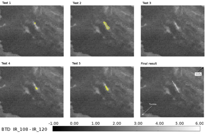
Fig. 09. Test 1–Test 5: Background, BTD image (in K). Enclosed in yellow, guide points found in each test. Bottom, right: Output of Step I, line (white) that corresponds to the contrail tracked by ACTA. Table 03 shows the process in detail. Location: Over the Mediterranean between Sicily and Tunisia. Date: 19 June 2009 09:45 UTC.

Fig. 9. Test 1–Test 5: Background, BTD image (in K). Enclosed in yellow, guide points found in each test. Bottom, right: Output of Step I, line (white) that corresponds to the contrail tracked by ACTA. Table 3 shows the process in detail. Location: Over the Mediterranean between Sicily and Tunisia. Date: 19 June 2009 09:45 UTC.

Fig. 010.Schematic representation of Step II. Fig. 10. Schematic representation of Step II.

w1= 2 pixels,w2= 10 pixels, CRIT>max{mS·0.77,1}(K),

Acceptance criterion:R >0.98

Figure 6 shows an example of how ACTA works in the Test 3. In this case, Tests 1 and 2 have failed because of surrounding cloudiness and a second contrail crossing the scene. First, the contrailC(t )(Fig. 6a) is used as input to define a region within which contrail C(t0=t+1t ) could exist (Fig. 6b), then, the image is filtered (Fig. 6c) to enhance contrail fea-tures and the tests are run to look for the guide points in the allowed region (Fig. 6d). Once the guide points are found

Table 3. Example of ACTA’s Step I.am(t )= −1.36,bO: orienta-tion, A: alignment. Due to the characteristics of the contrail, only Test 5 provides a satisfactory output to continue the tracking.

Test Number of Correlation Slope Acceptance guide points coefficient m0a criterionb

1 1 – – O

2 17 0.954 −1.58 A

3 0 – – O

4 2 1 −1 A and O

5 5 0.989 −1.65 A

(Fig. 6e), a linear fit is performed (Fig. 6f). Note that an alien pixel not belonging to the contrail is present as guide point. If the resulting line fulfils the orientation criterion, this line then is used as input line for the following timeslot and ACTA can proceed to Step II. Otherwise, ACTA performs Test 4.

(9)

Fig. 011.Process of selecting the contrail pixels. (a) Original BTD image. (b) Line from Step I. (c) Mask labeling the pixels around the line that lie within a given distance,Dij. (d) Mask combining the distance information and the BTD signal, BTDij·Dij. (e) Mask containing

information about the maxima of each line of the image, DILij. (f) Pixels resulting after combining masksM1,M2andM3and performing

the clustering test.

Fig. 11. Process of selecting the contrail pixels. (a) Original BTD image. (b) Line from Step I. (c) Mask labeling the pixels around the line that lie within a given distance,Dij. (d) Mask combining the distance information and the BTD signal, BTDij·Dij. (e) Mask containing

information about the maxima of each line of the image, DILij. (f) Pixels resulting after combining masks M1, M2and M3and performing the clustering test.

2.2 Step II: contrail shape

Once the position of the line is established, ACTA’s next step is to retrieve the contrail shape by selecting the pixels that also belong toC(t+1t )from the surroundings of the line. This is achieved by combining three different masks2 con-taining different information about the image and the posi-tion of the contrail. This Step combines the informaposi-tion of the line derived in Step I with the BTD image. Step II fo-cuses on the neighbourhood of the line (Mask 1), identifies the edges of the contrail (Mask 2) through filtering, and out-lines a possible shape by selecting the pixels with a higher BTD (Mask 3). A final clustering test retrieves the shape by selecting the pixels in groups. Figure 10 outlines the process followed by Step II. It is important to point out that Step II identifies also the parts ofC(t+1t )that are not linear.

A complete definition of each mask in Step II and a step-by-step example (see Fig. 11) follow.

First mask: distance and BTD3

A first mask is built considering a neighbourhood of 4 pix-els around the line (see Fig. 11c). All pixpix-els on the neigh-2_{Mask: template image used to accept or reject patterns in}

an-other image under study. Each pixel in a binary mask accepts (1) or rejects (0) a pixel in the studied image

3_{Masks M}

1, M2, M3and Mfinal are matrices ofNi×Nj

ele-ments. Multiplication (·) involving these masks implies Hadamard (or Schur) product (elementwise multiplication of their elements)

bourhood are likely to belong to the contrail, constituting a distance mask.

The mask is thus 9 pixels wide, allowing the contrail to exist not only along the line, but within a radius of 16–20 km (latitude and longitude dependent) around the line. This en-ables the contrail to expand, to split and to lose linearity. The neighbourhood is implemented as a matrix, Dij, as follows:

Dij=

4 X

d=0

L(i±d,j±d) (6)

where L(i,j )is as defined in Step I, Eq. (1).

This distance mask is multiplied by the brightness temper-ature difference image. The result can be seen in Fig. 11d. The resulting mask, M1contains information from both the distance to the original line and the BTD. This allows the contrail to have nearly any shape within the boundaries of the neighbourhood. Only pixels having a positive signal in M1can belong to the contrail.

M1= (

1 , if BTDij·Dij>0

0 , otherwise (7)

Second mask: edge detection

(10)

1098 M. Vazquez-Navarro et al.: ACTA 24 M. Vazquez-Navarro et al.: ACTA

Fig. 012.Top: Laplacian of Gaussian filter applied, on a 16×16 grid, withσ = 2. Bottom: Left: BTD image corresponding to 17 June 2009 07:00 UTC covering part of the North Sea, northern Germany and western Denmark. Right: in orange, edges identified when applying LoG filter to the BTD image.

Fig. 12. Top: Laplacian of Gaussian filter applied, on a 16×16 grid, withσ=2. Bottom: Left: BTD image corresponding to 17 June 2009 07:00 UTC covering part of the North Sea, northern Germany and western Denmark. Right: in orange, edges identified when ap-plying LoG filter to the BTD image.

pixels. This second mask is also binary and assigns 0 to the edge pixels and 1 to the pixels not belonging to edges.

The edge detection algorithm is based on the Laplacian of Gaussian (LoG) filter described in Canty (2007). The computation of the gradient of a grey-scale image provides a maximum at an edge. The second derivative is zero at that maximum and has opposite signs immediately on either side. Thus, it is possible to determine edge positions to the accu-racy of one pixel by using second derivative filters.

Laplacian filters have the property of returning 0 in regions of constant intensity and in regions of constantly varying in-tensity but nonzero at their onset or end. They are also very sensitive to image noise, so first a Gaussian filter must be ap-plied to smooth the image. Since the convolution operation (∗) is associative, the application of both filters consecutively on the image is equivalent to calculating the Laplacian of the Gauss function and then using the resulting function as filter.

The Gauss function,G, in two dimensions is given by:

G= 1

2π σ2exp

− 1

2σ2(x 2 1+x22)

, (8)

where the parameterσ determines its width. Applying the Laplacian operator, the final filter is thus:

∇2G= 1

2π σ6(x 2 1+x

2 2−2σ

2_)exp₋ 1 2σ2(x

2 1+x

2 2)

. (9)

Let BTDf_ijbe the result of the convolution of the Laplacian of Gaussian filter, LoGij= ∇2G(x1,x2), with the BTD image:

BTDf_ij=BTDij·LoGij (10)

As the signs are opposite on either side of the edge, the zero crossings in the horizontal and vertical directions are deter-mined from the products of the image with a copy of itself shifted by one pixel to the right and upward, respectively. Let BTDf,_ijupand BTDf,_ijright be the filtered BTD images shifted upwards and rightwards, respectively. Sign changes corre-spond to negative values in the products and these define the edges, Eij.

F1ij=BTDf_ij·BTDf,_ijup

F2ij=BTDfij·BTD f,right

ij

Eij=

(

1 , where F1ij<0 ∨ F2ij<0

0 , otherwise (11)

Finally,

M2= (

0 ,∀(i,j )|Eij=1

1 , otherwise (12)

Figure 12 shows the filter applied in this work (size: 16×16 pixels andσ=2) and an example of the identified edges.

Third mask: maxima

The contrail corresponds to the pixels in the BTD image with a larger brightness temperature difference. This mask in-tends to identify the pixels that have a stronger BTD signal and their surroundings, that is, this mask retrieves a possi-ble shape of the contrail. To locate the pixels that present a larger BTD, first the pixel with the strongest BTD signal in each horizontal line within the neighbourhood area (see Eq. 7) is selected:

MAXij=

(

1 , if BTDij=maxi0≤k≤iN(M1(k,j ))

0 , otherwise (13)

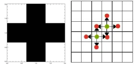
A broader region around the maxima is created expanding the pixels found up, down, left and right, as in the example below (Fig. 13, left).

Technically, this is carried out applying the morphologi-cal operator dilate4(Stark et al., 1998) to these pixels using 4_{Dilation (}_⊕_{), is the transformation of an image by a}

(11)

Fig. 13. Left: 3×3 structuring element used in the dilation. Black=1, White=0. Right: Example of creation of a broader re-gion. Green: original pixels. Green and red: expanded (dilated) region.

the cross-shaped 3×3 pixel structuring element, STRUCTij,

shown in Fig. 13, right

DILij=MAXij⊕STRUCTij (14)

An example of the resulting image, DILij, can be seen in

Fig. 11e. Next, the temperature difference of the pixels in DILij is calculated and compared with the average of the

brightness temperature difference in the original area, Dij

(Fig. 11c, Eq. 6). Due to the fact that allowed region in Dij

is very wide, most of the pixels in it (water clouds or surface) have a low BTD signal whereas only a few (either only the contrail or the contrail and cirrus clouds nearby) will have a strong BTD signal. Let the average BTD in Dij be BTD. The

pixels having a lower temperature difference than BTD, i.e. a weaker BTD signal, are assigned a zero likelihood of be-ing contrail pixels. This way, the mask can discard the pixels with a lower-than-average BTD, a scene-dependent criterion that points out the contrail pixels on the image. The result constitutes the third mask (see Eq. 15).

M3= (

1 ,∀(i,j )∈DILij | DILij·BTDij>BTD

0 ,otherwise

(15)

Combination of masks

By combining the three masks with a logical AND: the mask containing information both from the proximity to the line and from the temperature difference, the mask derived from the edge detection algorithm, and the mask resulting from applying the dilate operator to a selection of the stronger sig-nal pixels and refining the result, a fisig-nal binary mask can be obtained. Pixels where Mfinal=1 are labeled as possible con-trail pixels:

Mfinal=M1·M2·M3 (16)

Clustering

The labeled pixels undergo a final clustering test to identify the grouped regions and discard isolated ice cloud pixels that have been misidentified in Mfinal. A contrail is typically a connected region sometimes split into smaller areas. Only the pixels belonging to connected regions of more than 3 con-tiguous pixels are considered contrail pixels.

In this work, the IDL command label region has been used. Let CLij =cluster(Mfinal)the result of applying la-bel region to the two-dimensional array Mfinal. CLij, is an

array of the same dimensions as Mfinal where each cluster carries a consecutive numeric label. Therefore, pixels in Cluster 1 haveCL=1, pixels in Cluster 2,CL=2, etc. Let mCL=max(CLij)be the number of clusters or connected

regions in Mfinal. The number of pixels,np, in each cluster, p, is:

np=i,j∈Mfinal | clij=p (17)

Thus, the contrail pixels con px can be defined by:

con px=i,j∈clij|np>3 , 0< i < mCL (18)

The pixels selected as contrail pixels by ACTA are shown on Fig. 11 (bottom, right): all pixels enclosed by the yellow line are contrail pixels. This example also shows that the presence of a secondary contrail very close to the tracked contrail does not affect the final result. The westernmost and easternmost pixels±10 pixels are used as limitsi0andi1for the length of the contrail in Step I.

When the Step II of ACTA is over and the whole set of pixels that corresponds to contrail C(t+1t ) is identified, ACTA writes the position of the contrail pixels to a file and proceeds to Step I using the line parameters ofC(t+1t )as input for the following time slot.

3 Example

(12)

Fig. 014.Slope(a)and intercept(b)of the line defining the contrail (y=ax+b) in each moment of its development. The level of gray indicates the age of the contrail.

Fig. 14. Slope (a) and intercept (b) of the line defining the contrail (y=ax+b) in each moment of its development. The level of gray indicates the age of the contrail.

The example here presented corresponds to the 5 April 2009. The contrail drifted over the bay of Biscay and has been tracked for 6 h and 30 min. The MODIS overpass at 11:35 UTC allowed the CDA to detect this linear contrail north of Spain. ACTA used the SEVIRI 5-min Rapid Scan data to track it back to 11:00 UTC and forth until 17:35 UTC. Figure 16, see supplement, shows the results. The yellow line encloses the pixels that ACTA has identified as contrail. The vicinity of other contrails parallel to the tracked one does not affect the tracking and that neither the crossing over a pre-existing contrail nor the presence of underlying cloudiness lead to a misidentification of the original contrail.

After two hours, the contrail has lost the distinct linear fea-ture and is no longer recognisable as such had it not been for its previous history. The input provided by the CDA corre-sponds to 11:35 UTC and is marked with a blue frame. The temporal resolution is 5 min.

To show that the tracking always identifies the same con-trail the following two figures have been included: the rela-tionship between slope and intercept that ACTA has used to identify the position of the contrail in each timeslot in Step I shows a very smooth change (see Fig. 14). Moreover, the area covered by the contrail does neither show any blank spaces nor a motion against the wind field (see Fig. 15).

4 Summary and conclusions

ACTA is a tracking algorithm that identifies contrails and contrail-cirrus over a substantial part of their lifetime tak-ing advantage of the high temporal resolution of the SEVIRI sensor (5 min). The most important feature of ACTA is that the only information necessary to start the tracking of the contrail/contrail-cirrus is a single positive identification at

Fig. 015. Area covered by the contrail during the tracking. The level of gray indicates the age of the contrail.

Fig. 15. Area covered by the contrail during the tracking. The level of gray indicates the age of the contrail.

any stage of its development. Here we used the CDA ap-plied to MODIS data, but any other reliable identification of a contrail can serve as a starting point for ACTA such as data input from a human observer or any other instrument with a high spatial resolution.

ACTA’s results have been visually verified in a large num-ber of cases. It has been confirmed that the performance of the algorithm is excellent with rapid-scan data, where the temporal delay between successive images is five minutes. Larger time steps such as the regular 15 min scan can be used for isolated contrails, but in a scene with many parallel lin-ear contrails, ACTA might misidentify the contrail. In these cases it may select a neighbouring contrail to continue the tracking.

According to the design of ACTA it is not necessary to use actual wind field data. Use of ECMWF wind field data has not improved the accuracy of the tracking but resulted in much longer processing times. Considering a wind speed of 110 km/h (∼60 knots) at 10 km height and using it to define the region within which the contrail can move each 5 min is sufficient for the tracking and has reduced significantly the computing time and the logistic effort of including another dataset. ACTA is very fast, each iteration requires in average less than one minute on a usual desktop machine. The actual time required is dependent on the number of tests that must be performed in Step I.

ACTA uses only two SEVIRI channels, IR 108 and IR 120. Additional channels or channel combinations have been considered, such as the IR 039 (3.9 µm) for discriminat-ing between water and ice clouds or water vapour channels WV 062 (6.2 µm) and WV 073 (7.3 µm), and also BTDs in-volving IR 087 (8.7 µm), but these considerations have not added significant improvements to the result while notably increasing the computation time.

(13)

M. Vazquez-Navarro et al.: ACTA 1101 satellite instrument: the early stages, with sub-pixel width

or low optical thickness and low contrast with the surround-ings; and at the end of the life cycle, when the contrail again becomes optically thin or cannot be any longer discriminated from the surrounding, which might be also influenced by air traffic. These are ACTA’s known limitations. ACTA provides considerably more information than the CDA algorithm but may still miss part of the evolution of contrails and contrail-cirrus.

If the input does not provide the full length of a contrail, some contrail pixels are initially ignored. To prevent this, ACTA has loose boundary conditions that allow the tracked cloud to be longer or shorter than suggested by the input data, correcting the length of the contrail/contrail-cirrus in subse-quent intervals. Nevertheless, an input contrail that is too short can result in a too short tracked contrail. This problem can be solved using a human input, i.e. if the researcher feeds ACTA with input line parameters detected visually. Thus, throughout the lifetime of the contrail its full length can be accurately tracked. The objective of this work was to per-form a statistical analysis over a very large number of con-trails, so human input was not considered to be a feasible option. For each time step, an average value of all pixels is used for further analysis, so ignoring a few contrail pixels in certain scenes due to the automatic input does not imply a substantial change in the average when computing lifetime, or other physical properties such as optical thickness or ra-diative forcing. The combination of ACTA and CDA pro-vides such a large number of occurrences that the occasional omission of pixels can be considered negligible. Besides, this work aims to establish a minimum value for the effect of anthropogenic aviation clouds on the climate system. Of extreme importance is that all pixels labeled as contrail pix-els actually belong to contrails. This point has been fulfilled satisfactory by ACTA.

The CDA has a low but non-zero false alarm rate. The detected contrails are mapped by ACTA on the MSG grid and tracked. The different performance and spatial resolu-tion of the instruments and algorithms involved can lead to two different types of errors. In the first place, features mis-detected by the CDA have to be eliminated. Second, since CDA and ACTA data work on different spatial resolutions, it is possible that the CDA detect a very narrow contrail on the MODIS scene (resolution 1 km) that cannot be detected by the SEVIRI sensor (pixel size at least 3×3 km).

Supplementary material related to this article is available online at:

http://www.atmos-meas-tech.net/3/1089/2010/

amt-3-1089-2010-supplement.amt-2010-35-supplement. zip.

Acknowledgements. This research was supported by the

European Union FP6 Integrated Project QUANTIFY (http://www.pa.op.dlr.de/quantify/) and by the “Climate-compatible Air Transport System” (CATS) DLR project. We would like to thank U. Schumann (DLR) for his support and helpful comments and H. Volkert (DLR) for his constructive suggestions.

Edited by: A. A. Kokhanovsky

References

Bakan, S., Betancor, M., Gayler, V., and Graßl, H.: Contrail fre-quency over Europe from NOAA-satellite images, Ann. Geo-phys., 12, 962–968, doi:10.1007/s00585-994-0962-y, 1994. Canty, M. J.: Image analysis, classification and change detection in

remote sensing, CRC Taylor & Francis, 2007.

Fu, Q. and Liou, K. N.: Parameterization of the Radiative Properties of Cirrus Clouds, J. Atmos. Sci., 50, 2008–2025, 1993. Gierens, K.: Numerical simulations of persistent contrails, J.

At-mos. Sci., 53, 3333–3348, 1996.

Lee, D. S., Fahey, D. W., Forster, P. M., Newton, P. J., Wit, R. C. N., Lim, L. L., Owen, B., and Sausen, R.: Aviation and global climate change in the 21st century, Atmos. Environ., 43, 3520– 3537, doi:10.1016/j.atmosenv.2009.04.024, 2009.

Lee, T. F.: Jet contrail identification using the AVHRR infrared split window, J. Appl. Meteorol., 28, 993–995, 1989.

Mannstein, H., Meyer, R., and Wendling, P.: Operational Detection of Contrails from NOAA-AVHRR-Data, Int. J. Remote Sens., 20, 1641–1660, 1999.

Meyer, R., Mannstein, H., Meerkoetter, R., Schumann, U., and Wendling, P.: Regional radiative forcing by line-shaped contrails derived from satellite data, J. Geophys. Res., 107(D10), 4104, doi:10.1029/2001JD000426, 2002.

Meyer, R., Buell, R., Leiter, C., Mannstein, H., Marquart, S., Oki, T., and Wendling, P.: Contrail observations over Southern and Eastern Asia in NOAA/AVHRR data and comparisons to con-trail simulations in a GCM, Int. J. Remote Sens., 28, 2049–2069, 2007.

Minnis, P., Palikonda, R., Walter, B. J., Ayers, J. K., and Mannstein, H.: Contrail properties over the eastern North Pacific from AVHRR data, Meteor. Z., 14, 515–523, 2005.

Palikonda, R., Minnis, P., Duda, D. P., and Mannstein, H.: Contrail coverage derived from 2001 AVHRR data over the continental United States of America and surrounding areas, Meteor. Z., 14, 515–523, 2005.

Ponater, M., Marquart, S., and Sausen, R.: Contrails in a com-prehensive global climate model: parameterization and ra-diative forcing results, J. Geophys. Res, 107(D13), 4164, doi:10.1029/2001JD000429, 2002.

Schumann, U.: Formation, properties and climatic effects of con-trails, C. R. Physique, 6, 549–565, 2005.

Stark, J.-L., Murtagh, R., and Bijaoui, A.: Image Processing and Data Analysis. The multiscale approach, Cambridge University Press, 1998.