R E S E A R C H
Open Access
Tree-average distances on certain phylogenetic
networks have their weights uniquely determined
Stephen J Willson
Abstract
A phylogenetic networkNhas vertices corresponding to species and arcs corresponding to direct genetic inheritance from the species at the tail to the species at the head. Measurements of DNA are often made on species in the leaf set, and one seeks to infer properties of the network, possibly including the graph itself. In the case of phylogenetic trees, distances between extant species are frequently used to infer the phylogenetic trees by methods such as neighbor-joining.
This paper proposes atree-averagedistance for networks more general than trees. The notion requires aweighton each arc measuring the genetic change along the arc. For each displayed tree the distance between two leaves is the sum of the weights along the path joining them. At a hybrid vertex, each character is inherited from one of its parents. We will assume that for each hybrid there is a probability that the inheritance of a character is from a specified parent. Assume that the inheritance events at different hybrids are independent. Then for each displayed tree there will be a probability that the inheritance of a given character follows the tree; this probability may be interpreted as the probability of the tree. Thetree-averagedistance between the leaves is defined to be the expected value of their distance in the displayed trees.
For a class of rooted networks that includes rooted trees, it is shown that the weights and the probabilities at each hybrid vertex can be calculated given the network and the tree-average distances between the leaves. Hence these weights and probabilities are uniquely determined. The hypotheses on the networks include that hybrid vertices have indegree exactly 2 and that vertices that are not leaves have a tree-child.
Keywords:digraph, distance, metric, hybrid, network, tree-child, normal network, phylogeny
1 Introduction
In phylogeny, the evolution of a collection of species is modelled via a directed graph in which the vertices are species and the arcs indicate direct descent, usually with modification as mutations accumulate. The leaves typi-cally correspond to extant species, while internal vertices typically correspond to presumed ancestors. It has been common to assume that the directed graphs are trees, but more recently more general networks have also been studied so as to include the possibility of hybridi-zation of species or lateral gene transfer. General frame-works for phylogenetic netframe-works are discussed in [1], [2], [3], and [4]. See also the recent book [5].
There are many methods to reconstruct phylogenetic trees from information such as the DNA of extant spe-cies. The most generally accepted methods include
maximum parsimony, maximum likelihood, and Baye-sian. See [6] for an overview. These methods, however, are only heuristic, do not guarantee an optimal solution, and can be very time-consuming for a moderate number of species.
SupposeX denotes the set of extant species for some analysis, including an outgroup which is used to locate the root. The DNA information may be summarized via the computation of distances between members of X. If
x,y ÎX, thend(x,y) summarizes the amount of genetic difference between the DNA strings ofxand y. In order to compensate at least partially for the possibility of repeated mutation at the same site, a number of differ-ent distances are in use, based on differdiffer-ent models of mutation. Notable examples include the Jukes-Cantor [7], Kimura [8], HKY [9], and log determinant [10], [11] distances. The log determinant distance is especially interesting in that it can be proved that typically the Correspondence: swillson@iastate.edu
Department of Mathematics, Iowa State University, Ames, IA 50011 USA
distances add along the paths, so that the distance along a path is the sum of the distances for each edge along the path.
Some fast methods to reconstruct phylogenetic trees make use of distances between members ofX. Probably the most common distance-based method is Neighbor-joining [12]. It is computationally fast. It often gives a good initial tree with which heuristic methods begin in order to find an improved tree by other methods. Another more recent method FastME [13], [14] is based on the principle of balanced minimum evolution, in which one assumes that the correct tree is the one that exhibits the minimal total amount of evolution, suitably measured.
Distance-based methods have been rarely used to con-struct phylogenetic networks that are not necessarily trees. It is true that distances occur in common explora-tory methods to display the diversity of trees for the same species such as the split decomposition (see [15] or an overview in [5]). These distances, however, are not derived from any biologically based model of evolution.
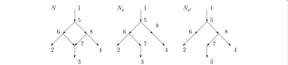
This paper studies a distance on rooted directed net-works that is based upon a model of evolution. Con-sider, for example, the networkNin Figure 1. The root is 1 and there is a hybridization event at 7 with parents 6 and 8. Vertex 7 is called ahybridvertex or a reticula-tionvertex. For some characters, the character state at 7 is inherited from the parental species 6, while for other characters the character state at 7 is inherited from spe-cies 8. For character states inherited from 6 the evolu-tionary history is best described by the displayed tree
Np, while for character states inherited from 8 the
his-tory is best described by the treeNp’. Herepandp’are parent mapstelling the parent of every non-root vertex. In the example p(7) = 6 while p’(7) = 8. Each parent mappleads to a displayed treeNp.
In Figure 1, each arc might have a numericalweight
measuring the amount of genetic change on the arc. In either treeNpor Np’the distance between two vertices might be plausibly defined as the sum of the weights of the edges on the unique path between the vertices. This
paper explores the possibility that an appropriate dis-tance between the vertices in the network N is a weighted average of the distances inNpandNp’.
More generally, the trees displayed by a network N
will be conveniently indexed as Npwherepranges over
all the parent maps. LetPar(N) denote the set of all par-ent maps forN. For each hybrid vertexh, the probability that a character ofh is inherited from a particular par-ent vertexqiwill be denoted a(qi, h). Assume that these
inheritances at different hybrid vertices are independent events. Then for eachp Î Par(N) we obtain that the probabilityPr(p) that the treeNpmodels the inheritance
of a particular character is given by
Pr(p) =[α(p(h), h) :his hybrid].
Ifx and y are vertices, then the distance between x
and y in Np, written d(x, y; Np), is the sum of the
weights of arcs on the unique path joining xand y in
Np. The tree-average distance d(x,y;N) betweenxandy
inNwill be defined to be the expected value of the dis-tances in the various treesNp:
d(x,y;N) =[Pr(p)d(x,y;Np) :p∈Par(N)].
If a hybrid vertex h satisfies that each parentq of h
has the same probability, we will call the inheritance
equiprobable at h. This special case assumes that the contribution from each parent to his the same; if there are two parents, each contributes approximately 50%.
In Figure 1 note that, for each species in the leafsetX
= {1, 2, 3, 4}, it is plausible that the DNA is available since 2, 3, 4 correspond to extant species and 1 to an extant outgroup species. Hence it is plausible that we knowd(x,y;N) for distinctx andyinX, hence 42= 6 nonzero distances. Nevertheless,Nhas 8 arcs and hence it is not likely that from the 6 known distances we could compute 8 independent weights for these arcs. Indeed, the equations obtained in this paper for this net-work have infinitely many solutions. There is a possibi-lity of simultaneous identical mutations between 6 and
? @
@ R @
@
R @@R ?
1
2
3
4 5
6
7 8
N
? @
@ R @
@
R @@R ?
1
2
3
4 5
6
7 8
Np
? @
@ R
@ @ R ?
1
2
3
4 5
6
7 8
Np
7 and between 8 and 7 which might be confused with mutations between 7 and 3.
In this paper we will assume that the weight of an arc into a hybrid vertex is 0. Thus in Figure 1, the weights of arcs (6, 7) and (8, 7) will be zero. Under this assump-tion vertex 7 corresponds roughly to the immediate off-spring of a hybridization event, in which some characters came intact from 6 and the remainder intact from 8. Further mutation occurred before species 3 evolved from 7.
Note that the number of arcs ofNin Figure 1 that are not directed into a hybrid vertex is 6. It is therefore plausible that given the 6 numbers d(x,y;N) forx, yÎ
{1, 2, 3, 4}, we might be able to recover the weights for each of the 6 arcs inN that are not directed into the hybrid vertex 7. These same weights would be utilized in distances for bothNpandNp’. On the other hand, we
should like to determine an additional parametera(6, 7) telling the probability of inheritance by 7 of a character from 6. It is unlikely that six equations, one for each d
(x, y; N), will uniquely and generically determine seven real parameters. Indeed, the methods of this paper for this example lead to six equations in seven unknowns such that for certain values of the distances the weights and probabilities are not uniquely determined. Conse-quently for the situation in Figure 1 we will assume that
a(6, 7) =a(8, 4) = 1/2; we call the inheritance equiprob-able at 7.
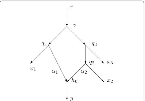
By contrast, Figure 2 shows another network withX= {r,x1, x2,x3, y} containing a single hybrid vertexh0. In this case there are 52= 10 distances and 8 arcs not into a hybrid vertex, so it is plausible that the 10 equa-tions would allow us to uniquely determine a ninth parametera1 =a(q1, h0) satisfying 0 <a1 <1. In fact, this paper will show how to determine all 9 parameters.
Thena(q2,h0) = 1 -a1 is also determined. In Figure 2
we will not need to assume equiprobability ath0. In order to obtain interesting results, assumptions must be made about the networkN. As an extreme case it would be easy to add many more internal vertices and edges to the network Nof Figure 1 without adding any additional leaves yet increasing arbitrarily the number of arcs. For example, Figure 3 shows a network in which the network N of Figure 1 has been modified by the addition of other arcs. The 6 distances do not determine the weights for all 7 arcs that do not lead to a hybrid vertex in Figure 3.
Particular kinds of acyclic networks have been studied in various papers. Wang et al. [16] and Gusfieldet al. [17] study “galled trees” in which all recombination events are associated with node-disjoint recombination cycles; the idea occurs also earlier in [18]. Choyet al. [19] and Van Iersel et al. [20] generalized galled trees to
“level-k“networks. Baroni, Semple, and Steel [2] intro-duced the idea of a“regular”network, which coincides with its cover digraph. Cardona et al. [21] discussed
“tree-child”networks, in which every vertex not a leaf has a child that is not a reticulation vertex. An arc (a, b) isredundantif there is a directed path fromato b that that does not utilize this arc. The current author has utilized “normal” networks [22] which are both tree-child and contain no redundant arc.
Most results in this paper assume that the network is
normal. This means, briefly, that every vertex not inX
and not a leaf has a tree-child (a child with indegree one); and moreover, there is no redundant arc. For example, ifX= {1, 2, 3, 4} then the network in Figure 1 is normal while the network in Figure 3 is not normal since arc (5,10) is redundant. With the assumption that
? @
@ @ R
@ @
@ R ? @
@ @ R A
A A
A A
AU
?
r
x1
y
x2
x3
v
q1 q3
α2
α1
q2
h0
Figure 2A minimal configuration needed to be able to find the probabilitya1=a(q1,h0) = 1-a2that a character state in
h0is inherited fromq1.
? @
@ @ R
? ?
@ @
@ R
@ @
@ R
?
1
2
3
4 5
6
7
8 9
10
there are no redundant arcs we show in Section 3 that for a given networkN, the tree-average distance dis a metric onX. With the assumption of normality we also show that different parent maps pyield different dis-played trees Np. Hence the average over the parent
mapspis the same as the average over displayed trees. This result eliminates the logical possibility that differ-ent pardiffer-ent maps p1 and p2 might yield displayed trees that are topologically the same, yielding an uncertainty about which is the correct average to use in the definition.
The main result, Theorem 4.1, assumes that the net-work Nis normal and also that for all hybrid vertices the indegree is exactly 2 and the outdegree is exactly 1. At each hybrid vertexhwe assume either equiprobabil-ity or else thathhas a grandparent on at least one side of the reticulation cycle, as in Figure 2 but not Figure 1. Then from knowledge both ofNand of the tree-average distance function d, the weights for all arcs are uniquely determined and indeed can be computed by explicit for-mulas. Moreover, the probabilities of inheritance at each hybrid vertex are uniquely determined and can be com-puted by explicit formulas. This calculation is, of course, trivial if the network is equiprobable ath.
A model for a distance function containing certain parameters is calledidentifiable if the parameters can be reconstructed from the (exact) values of the distance function. Theorem 4.1 thus asserts that, if the tree-aver-age distance function d on X and the network N are known, then the real parameters of the model (i.e., the weights and the probabilities) are identifiable in various cases.
A major problem, of course, is the reconstruction ofN
itself from a distance functiond. I have obtained partial results (not included in this paper) which give a recon-struction of N itself when the distance d is the tree-average distance and when the networkNsatisfies the hypotheses of Theorem 4.1 and some additional hypoth-eses. The reconstruction of Nis possible because of the simple forms of the formulas obtained in this paper. Essentially, the formulas are simple enough that they can be used recursively when only part of the network is yet known. I plan a subsequent paper which will uti-lize the results in the current paper to reconstruct N
from the tree-average distances.
The assumption that all hybrid vertices have indegree 2, assumed in Theorem 4.1, is plausible biologically since in sexually reproducing species an offspring arises from one egg and one sperm.
The assumption that there be no redundant arcs is essential for Theorem 4.1. Figure 3 displays a tree-child network NwithX = {1, 2, 3, 4}. There are 6 indepen-dent nonzero distances between the members ofX, yet there are 7 arcs not directed into hybrid vertices. It is
easy to choose positive values for the tree-average dis-tances such that there are infinitely many positive choices of the weights given the network. Note that each vertex not a leaf has a tree-child, so the network is a tree-child network [21]. Hence Theorem 4.1 cannot be extended to general tree-child networks.
Some other extensions of the current results and pro-blems are discussed in the concluding section 6.
2 Fundamental Concepts
A directed graph or digraph (V, A) consists of a finite setVof verticesand a finite setAofarcs, each consist-ing of an ordered pair (u,v) where uÎ V,vÎ V, u≠ v. We interpret (u, v) as an arrow fromu tovand say that the arcstartsat uandends atv. There are no mul-tiple arcs and no loops. If (u,v)ÎA, say thatuis a par-ent of v and v is a child of u. A directed path is a sequenceu0,u1, ...,ukof vertices such that for i= 1, ..., k, (ui - 1,ui)ÎA. The path istrivialifk= 0. Write u≤ vif there is a directed path starting at uand ending at
v. The digraph isacyclicif there is no nontrivial directed path starting and ending at the same point. If the digraph is acyclic, it is easy to see that ≤ is a partial order onV.
The indegreeof vertexu is the number ofvÎ Vsuch that (v,u)ÎA. The outdegreeofuis the number ofvÎ Vsuch that (u,v)Î A. Aleafis a vertex of outdegree 0. A normal vertex(ortree vertex) is a vertex of indegree 1. Ahybridvertex (orreticulation vertex) is a vertex of indegree at least 2. An arc (u,v) is anormal arcifvis a normal vertex.
A digraph (V,A) isrootedif it has a unique vertexr Î Vwith indegree 0 such that, for allvÎ V, r ≤ v. This vertexr is called theroot.
LetX denote a finite set. Typically in phylogeny,Xis a collection of species. Measurements are assumed to be possible among members ofX, so that we may assume that, for example, their DNA is known for eachxÎX.
A phylogenetic X-network N= (V,A, r, X) is a rooted acyclic digraph G= (V, A) with root rsuch that there is a one-to-one mapj: X ®V whose image contains all verticesvsuch that either
(i)vis a leaf; or (ii)v=r; or
(iii)vhas indegree 1 and outdegree 1.
There may be additional vertices inX. We will identify eachxÎ Xwith its image j(x). The setX will be called thebase-setforN.
In biology the network gives a hypothesized relation-ship among the members ofX. It is quite common also that a certain extant outgroup speciesr’ is assumed to have evolved separately from the rest of the species in question. When this happens, we identify the speciesr’
by (i) since measurements can be made on them. The outgroupr’, which is identified with the root, is inX by (ii). If a vertex has indegree 1 and outdegree 1 then nothing uniquely determines it unless, for fortuitous reasons, it is possible to make measurements on its DNA, in which case it lies in the base-setX.
AnX-tree is a phylogeneticX-network such that the underlying digraph is a tree.
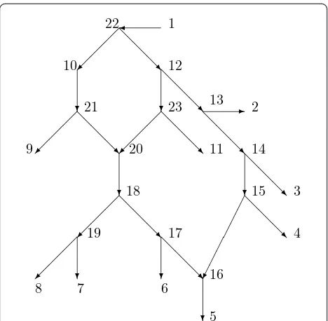
Figure 4 shows a phylogeneticX-networkNwith base-setX= {1, 2, 3, 4, 5, 6, 7, 8, 9, 10, 11}. The root isr= 1. Note that the leaves are inXby (i), 1ÎX by (ii), and 10
Î X by (iii). Measurements such as DNA are assumed possible on members ofX. Since the root 1 is actually an outgroup and the leaves are all extant, this is plausi-ble for all members of X except 10. We are perhaps here assuming that, by some fortuitous chance, some historical DNA of 10 is also available.
An arc (u, v)Î Aisredundant if there existswÎ V
such that u, v, and ware distinct and u≤ w ≤ v. The removal of a redundant arc (u, v) still leavesu ≤ vin the network.
A phylogenetic X-network N = (V, A, r, X) with base-set X isnormalprovided (1) whenever vÎ Vand
v ∉X, then v has a tree-childc; and (2) there are no redundant arcs. The networks in Figure 2 and 4 are normal, while the network of Figure 3 is not normal. The usage here of“normal” differs slightly from that in [22] in that here hybrid vertices that are not leaves may have outdegree 1, whereas in [22] hybrid vertices
that were not leaves had outdegree 2 or higher. There is an obvious one-to-one relationship between normal networks in the current sense and normal networks in the previous sense.
A normal networkNissemibinary if each hybrid node has indegree 2 and outdegree 1. It follows from normal-ity that the child of the hybrid node is necessarily normal.
Anormal path inNfromvtoxis a directed pathv=
v0, v1, ...,vk=x such that fori= 1, ... k, vi is normal. A normal path from v to Xis a normal path starting at v
and ending at somexÎX. For example, in Figure 4, the path 20, 18, 19, 8 is normal and is a normal path from 20 toX. The path 18, 17, 16, 5 is not normal since 16 is hybrid. The trivial path 3 is normal.
SupposeNis normal andvÎV. Then there is a nor-mal path fromvtoX. To see this, ifvÎX, then the tri-vial path is a normal path fromvtoX. Ifv∉X, thenv
has a tree child v1. If v1 Î X, then the pathv0, v1 is a normal path tov1 inX. Otherwisev1 has a tree-childv2. If v2 Î Xthen the path v0, v1,v2 is a normal path from
vtov2 in X. Proceeding in this manner, we obtain the result.
Suppose two normal paths shared a common vertex x, say the normal pathsv=v0, ...,vk=xand w=w0, ...,wj
= x. If k >0 and j >0 then since x is normal with a unique parent, it follows that vk - 1 =wj - 1. Repeating
the argument we find that either there is an isuch that
v=wior else there is an isuch that w=vi. This
argu-ment, of frequent use, is called following the normal paths backwards.
Agraph(or, for emphasis, an undirected graph) (V,E) consists of a finite setVofvertices and a finite setE of
edges, each a subset {v1, v2} of Vconsisting of two dis-tinct vertices. Thus an edge has no direction, while an arc has a direction. If N= (V,A, r, X) is a phylogenetic
X-network, there is an associated undirected graphUnd
(N) = (V, E) in which every arc in Ahas its direction ignored; thusE= {{a,b}: (a,b)Î Aor (b,a)ÎA}.
3 The Tree-Average Distance
If N= (V, A, r, X) is a phylogeneticX-network, then a
parent map p for N consists of a map p: V -{r} ® V
such that, for all vÎ V- {r}, p(v) is a parent ofv. Note that r has no parent. If vis normal, then there is only one possibility for p(v), while ifvis hybrid, there are at least two possibilities for p(v). In Figure 4, an example of a parent mappsatisfies p(20) = 23,p(16) = 17, and for all other verticesvbesides 1,p(v) is the unique par-ent ofv.
WritePar(N) for the set of all parent maps forN. In general if there are kdistinct hybrid vertices and they have indegrees respectivelyi1,i2, ..., ik, then the number
of distinct parent mapspis |Par(N)| =∏[ij: j= 1, ...,
@
@ @ R
? ?
@ @
@ R @
@ @ R
@ @
@ R
? @
@ @ R
?
@ @
@ R ?
-@
@ @ R
? @
@ @ R
@ @
@ R
?
1
2
3
4
5 6
7 8 9
10
11 12
13
14
15
16 17 18
19 20 21
22
23
k]. IfNis a network withkdistinct hybrid vertices, each of indegree 2, then |Par(N)| = 2k.
GivenpÎPar(N) the set Apof p-arcsisAp= {(p(v), v): v Î V - {r}}. The induced tree Np is the directed
graph (V, Ap) with rootr. Note that each vertex inV
-{r} has a unique parent in Np. ThusNpis a tree with
vertex setV. The set X, however, need not be a base-set of Np. For example, if his hybrid in N, then inNp
the vertex hhas indegree 1 from the arc (p(h), h) and outdegree 1, yet need not lie inX.
Several of the proofs will require the notion of“ com-plementary parents”. Suppose pÎ Par (N) and his a particular hybrid vertex with exactly two parentsq1and
q2. Assume p(h) = q1. Thecomplementary parent map
p’ofp with respect to his defined by
p(v) =
p(v) ifv=h q2 ifv=h.
Thus p’ agrees with pexcept ath, where p’ chooses the other parent from that chosen byp.
A phylogenetic X-network is weighted provided that for each arc (a,b)Î Athere is a non-negative number
ω(a,b) called theweight of(a,b) such that (1) ifbis hybrid, thenω(a, b) = 0; (2) ifbis normal, thenω(a,b)≥0.
We call the function ω from the set of arcs to the reals theweight functionof N. We interpret ω(a, b) as a measure of the amount of genetic change from species
ato speciesb. If his hybrid with parentsq1andq2and unique childc, then the hybridization event is essentially assumed to be instantaneous betweenq1 andq2with no genetic change in those character states inherited byh
fromq1orq2respectively. Further mutation then occurs fromhtoc, as measured byω(h,c).
In any rooted tree T= (V,A, r), two vertices uandv
have a uniquemost recent common ancestormrca(u,v) = mrca(u,v;T)ÎVthat satisfies
(1) mrca(u,v)≤uand mrca(u,v)≤v;
(2) wheneverz≤uandz≤v, then z≤mrca(u,v). In a network that is not a tree, two vertices u andv
need not have a mrca(u,v).
Suppose thatN= (V, A, r, X) is a weighted phyloge-neticX-network with weight functionω. For eachpÎ Par(N) and for eachu, vÎV, define the distance d(u,
v; Np) as follows: in Np there is a unique undirected
pathP (u,v) between uand v; defined (u,v; Np) to be
the sum of the weights of arcs alongP(u,v). More pre-cisely, sinceNpis a tree, there exists a most recent
com-mon ancestor m = mrca(u, v; Np), a directed path P1 given by m = u0, u1, . . ., uk =u from m to u, and a
directed path P2 given bym=v0,v1, . . .,vj=vfromm
tov. Define
d(u,v;Np) = ω(ui,ui+1) :i= 0,· · ·,k−1
+ ω(vi,vi+1) :i= 0,· · ·,j−1
.
We shall refer tod(u,v;Np) as thedistance between u and v in Np.
LetHdenote the set of hybrid vertices ofN. For each
hÎ H, let P (h) denote the set of parents ofh, i.e. the set of vertices u such that (u, h)Î A. Since h Î H,|P
(h)|≥ 2. For eachuÎ P(h), let a(u,h) denote the frac-tion of the genome that h inherits from u. We may interpret a(u, h) as the probability that a character is inherited byhfromu, so for allhÎ H, ∑[a(u, h):uÎ P
(h)] = 1.
Ifhandh’are distinct members ofH, we will assume that the inheritances athandh’are independent. More generally, suppose for everyhÎHthatqhis a parent of h. Then we assume that the events that a character ath
is inherited from qh are independent. It is then easy to
see that for eachpÎPar(N) the probability that inheri-tance follows the parent map pisPr(p) =∏[a(p(h),h):
hÎH].
Thetree-average distance d(u, v; N) betweenuandv
inNis defined by
d(u,v;N) =[Pr(p)d(u,v;Np) :p∈Par(N)].
It is thus the expected value of the distances between
uandvin the variousNp.
The simplest situation has each parent of hequally likely, soa(p(h),h) = 1/|P (h)| for eachp ÎPar(N). If this situation occurs, we call the network equiprobable at h. If the networkNis equiprobable at hfor all h Î H, then we call the network equiprobable, and for each
uandvinX, d(u,v; N) is the average of the values d(u,
v;Np) forpÎPar(N).
For example, for the networkN in Figure 1 suppose that the arcs have weights given byω(1, 5) = 1 =ω(5, 6) =ω(7, 3), while ω(5, 8) = ω(8, 4) = 2 and ω(6, 2) = 4. Since 7 is hybrid,ω(6, 7) = ω(8, 7) = 0. Suppose, as in Figure 1, the parent mappsatisfies p(7) = 6 while the parent mapp’satisfiesp’(7) = 8. ThenNpshown in
Fig-ure 1 is obtained from Nby deleting the arc (8, 7) while
Np’ is obtained from N by deleting the arc (6, 7). Assumea(6, 7) = 1/3 anda(8, 7) = 2/3, soPr(p) = 1/3,
Pr(p’) = 2/3. To computea(1, 3;N) we findd(1, 3;Np)
=ω(1, 5) + ω(5, 6) +ω(6, 7) + ω(7, 3) = 1 + 1 + 0 + 1 = 3,d(1, 3;Np’) =ω(1, 5) +ω(5, 8) +ω(8, 7) +ω(7, 3)
= 1 + 2 + 0 + 1 = 4. Hence d(1, 3;N) = (1/3)d(1, 3;Np)
+ (2/3)d(1, 3; Np’) = (1/3)(3) + (2/3)(4) = 11/3. For
another exampled(1, 2; Np) = d(1, 2;Np’) = 6 so d(1, 2; N) = (1/3)(6) + (2/3)(6) = 6.
Givenu andv, the vertices mrca(u, v;Np) may differ
for differentp. This is seen in Figure 1 where mrca(2, 3;
Theorem 3.1. Assume N = (V, A, r,X) is a phyloge-netic X-network that has no redundant arcs. Assume N has a weight function ωsatisfying thatω(a,b)>0 if b is normal. Then the tree-average distance on X from N is a metric on X.
Proof. A metricdonX must satisfy
(1) For allxandyinX,d(x,y)≥0 and d(x,y) = 0 iffx
=y.
(2) For allxand yinX,d(x,y) =d(y, x). (3) For allx,y,zÎX,d(x,z)≤d(x,y) +d(y, z). For (2), suppose x,y,Î X. For allp, d(x,y; Np) =d(y, x;Np), whenced(x,y;N) =d(y,x;N).
For (3) supposex,y,zÎ X. For each Np, d(x, z;Np)≤ d(x,y;Np) + d(y,z; Np) from the truth of the four-point
condition, see [23], p 147. Hence the result follows for distances inNas well.
For (1) it is clear that for each p, d(x, y; Np) ≥ 0,
whenced(x,y;N)≥0. Moreover, for eachp, d(x,x; Np)
= 0, whenced(x,x; N) = 0.
To finish the proof of (1), suppose d(x,y; N) = 0; we showx=y. Assume insteadx≠y. Since the weights are nonnegative, for everypwe haved(x,y;Np) = 0. Hence
for everypÎ Par(N), inNpthe unique path betweenx
andy contains only arcs (a,b) withbhybrid inN. If x and y are both normal, then for every p the unique path between x and y in Np must consist of a
directed path from v= mrca(x, y; Np) to x and a path
fromvtoy; hence it contains a normal arc whenced(x,
y;Np)>0. Thus we may assume that one vertex, say y,
is hybrid.
InNchoose a directed path P=y0,y1, ...,yk=ysuch
that y1 is not hybrid but y2, ..., yk are hybrid. This is
always possible because there is a directed path fromr
to y, say u0=r,u1,u2, ..., uk=y. The childu1ofr can-not be hybrid, because if it were, then its other parent q
besides r must also have a path to q from r, and this path combined with the arc (q, u1) would make the arc
(r, u1) redundant. Moreover, we may choose this path
so that xdoes not lie in {y1, ..., yk} since whenever yiis
hybrid there are at least two choices of the parent yi -1,
and we may selectyi -1to be distinct fromx.
Ifx is normal in N, let Qbe the trivial path z0 =x. Otherwise we may choose a directed pathQ=z0, z1, ...,
zs=x such that z0 is not hybrid but all other vertices are hybrid. Moreover, we may assume that the vertices of Q are all distinct from the vertices of P . This is because, if zi is hybrid, it cannot have two parents q1 and q2which are onPsince then there must be a direc-ted path from say q1 to q2, whence the arc (q1, zi) is
redundant.
Since the vertices onP andQare distinct, there exists a parent mappthat agrees with all the choices made in constructing both P andQ. Hence in Np, P is a path
fromy0 toy,Qis a path formz0to x, and the paths are
disjoint. In Npletv= mrca(y0, z0;Np). Then in Npthe
unique path between x andy consists ofP , Q, a path
from vtoy0, and a path fromv toz0. Since y1 and z0
are normal, this path includes a normal arc, sod(x, y;
Np)>0. It follows thatd(x,y;N)>0, a contradiction.□
Corollary 3.2. Assume N is a normal network with weight function ω such that ω(a,b) >0 if b is normal. Then the tree-average distance on X from N is a metric on X.
The tree-average distance is defined as a weighted average in terms of parent maps. Any tree that arises as
Npfor some parent mappis said to bedisplayedin N.
There is a logical possibility that several different parent maps pcould yield essentially the same displayed tree. The next theorem gives sufficient conditions so that in fact the displayed trees are all distinct. Hence the tree-average distance becomes a weighted tree-average over all the distinct displayed trees.
The proof requires the notion of asplit. Asplit of Xis a partition of X into exactly two nonempty subsets; if these areAandB, we write the splitA|B. Two splitsA1|
B1 and A2|B2 are compatibleif at least one of the sets
A1∩ A2,A1∩B2,B1 ∩A2, andB1∩B2 is the empty set.
Removal of any edge e(but not its endpoints) from a treeTproduces a split ∑(e) consisting of vertices in the connected components ofTwith eremoved. The set of splits of a tree Twill be denoted ∑(T). IfT is directed, then the splits of T are obtained by reference only to the undirected tree so ∑(T) = ∑(Und(T)). By the Splits-Equivalence Theorem (see [23], p. 44) any two splits of a tree are compatible.
Theorem 3.3. Assume N = (V, A, r, X) is a normal phylogenetic X-network.Suppose that every hybrid vertex that is not a leaf satisfies that it has outdegree 1 and that its unique child is normal. Suppose p and q are dis-tinct parent maps for N. Then Npand Nq are topologi-cally distinct trees.
Proof. We show that ∑(Np) and ∑(Nq) are distinct.
Sincep≠qthere exists a hybrid vertex hsuch that p(h)
≠q(h). Letq1 =p(h) andq2 =q(h). Choose a normal path inNfrom q1 tox1 Î X, a normal path from q2 to
x2 Î X, and a normal path from htoy ÎX. Note that each normal path is a path in both Npand Nq.
More-over, q1 is normal inN because otherwise its unique child would not be a tree-child. Similarlyq2 is normal in
N.
If ∑(Np) = ∑(Nq), then each pair of splits would be
compatible. InNpconsider the split∑(a,q1) whereais
the unique parent of q1 and we remove the arc (a, q1) fromNp. We may write∑(a,q1) asA1|B1 whereA1 con-tainsr. The directed path inNpfromrto yincludes the
Npis rooted, there is a directed path from rtoq2. If it
included the arc (a,q1), then there would be a directed path in Np fromq1 to q2; this is not possible since in that case the arc (q1,h) would be redundant inN, con-tradicting normality ofN. SinceNpcontains the directed
path fromq2 tox2missing the arc (a,q1), it follows that
x2Î A1. Hence{r,x2}⊆A1and {y,x1}⊆B1.
InNq consider the split∑(b,q2) whereb is the parent
of q2 and we remove the arc (b,q2) fromNq. Similarly
to the case ofNpwe may write∑(b,q2) =A2 |B2 where {r, x1} ⊆ A2 and {y, x2} ⊆ B2. IfNp were topologically
the same asNq, then these splits would need to be
com-patible. Yet r Î A1 ∩ A2, x2 Î A1 ∩ B2, x1 Î B1 ∩ A2,
andy ÎB1∩B2, contradicting compatibility.□
Corollary 3.4. Suppose N= (V, A, r, X)is a phyloge-netic X-network that is normal. Suppose every hybrid vertex that is not a leaf has outdegree 1 and its unique child is normal. Suppose that there are exactly k hybrid vertices h1, h2, ..., hkand that for i= 1, ...,k, hybrid ver-tex hi has indegree di. Then the total number of distinct trees displayed by N and the total number of parent maps are both∏[di:i= 1, ...,k].
4 Finding the weight function fromd andN
In this section we prove the main theorem, that the weights are determined by knowledge ofNand the tree-average distances between members of X. For each hybrid vertexhwe will assume either equiprobability at
hor else a more complicated situation resembling Fig-ure 2. The assumptions can be different at different hybrid vertices.
Theorem 4.1. Suppose N= (V, A, r,X)is a phyloge-netic X-network which is normal and semibinary. Let ω be a weight function on A satisfyingω(a, b) = 0if b is hybrid andω(a,b)≥0 if b is normal. Assume that N is known and that the tree-average distance d(x, y; N)is known for each x and y in X.
For each hybrid vertex h with parents q1 and q2,
assume either
(1) the inheritance is equiprobable at h; or
(2) at least one parent (say q2) satisfies that there
exists q3such that
(a) there is a normal path from q3to q2;
(b) there is a normal path from q3 to some x3 in x
which is disjoint from the normal path from q3 to q2
except for the vertex q3;
(c) there is no directed path from q3to q1.
Then the weight function ω is uniquely determined and can be computed explicitly. Moreover, for each hybrid h, the probabilitiesa(qi,h)for each parent qiof h are uniquely determined and can be computed explicitly. See Figure 2 to understand the assumptions about h
in (2). Throughout this section we will assume the hypotheses of Theorem 4.1.
The proof primarily consists of a number of cases to handle different situations. We will present several of these special situations as lemmas and then later relate these together. Each lemma tells how certain distances or weights relate to distances between members ofX.
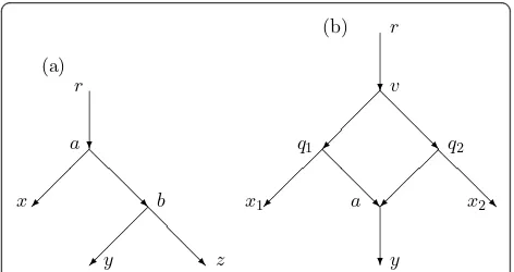
Lemma 4.2. Assume the hypotheses of Theorem 4.1. Suppose there is a normal path from a to b. Suppose there is a normal path from a to xÎ X which meets the normal path from a to b only in a. Suppose b has nor-mal paths to y and z in X which are disjoint except at b. Then d(a, b; N) = [d(r,y;N) +d(x, z;N)- d(r, x;N)- d
(y,z; N)]/2.
Proof. For eachpÎ Par(N), the path fromatob, the path from ato x, the path fromb to y, and the path fromb tozmust lie in Npsince none of the arcs enters
a hybrid vertex. Moreover, there must be a path fromr
to awhich includes none of the arcs on the other paths mentioned above. See Figure 5a. Hence for each pÎ Par(N) one can verify
d(r,y;Np) =d(r,a;Np) +d(a,b;Np) +d(b,y;Np)
d(x,z;Np) =d(a,x;Np) +d(a,b;Np) +d(b,z;Np)
d(r,x;Np) =d(r,a;Np) +d(a,x;Np)
d(y,z;Np) =d(b,y;Np) +d(b,z;Np).
It follows that
[d(r,y;Np) +d(x,z;Np)−d(r,x;Np)−d(y,z;Np)]/2 =d(a,b;Np).
Taking expected values we seed(a,b;N) =∑[Pr(p)d(a,
b;Np):pÎPar(N)] =∑[Pr(p)[d(r,y;Np) +d(x,z;Np)- d
(r,x;Np)- d(y,z;Np)]/2:pÎ Par(N)] = [d(r,y;N) +d(x, z;N)- d(r,x;N)- d(y;z;N)]/2.□
Lemma 4.3.Assume the hypotheses of Theorem 4.1.
(1) Suppose(a, b)is an arc where a ÎX and b is nor-mal. Suppose b has normal paths to y and z in X which are disjoint except at b. Then ω(a, b) = [d(a, y; N) +d
(a,z;N) -d(y,z;N)]/2.
? @
@ @ R @
@ @ R
@ @
@ R
?
r
x1
y
x2
v
q1
a
q2 (b)
? @
@ @ R
@ @
@ R
r
a
x b
y z
(a)
(2) Suppose there is a normal path from a to b Î X. Suppose there is a normal path from a to xÎ X which intersects the path from a to b only in a. Then d(a,b;N) = [d(b,r;N) +d(b,x;N)- d(r,x; N)]/2.
In particular, suppose (a, b)is an arc, bÎ X is nor-mal, and there is normal path from a to xÎ X which does not include b. Then ω(a, b) = [d(b,r; N) +d(b,x;
N)- d(r,x; N)]/2.
(3) Suppose(a, b)is an arc and b is normal. Suppose there is a normal path from a to xÎ X which does not include the vertex b. Suppose b has normal paths to y and z in X which are disjoint except at b. Then ω(a,b) = [d(r,y;N) +d(x,z;N)- d(r,x;N)- d(y, z;N)]/2.
Proof. For (1) we take a=x in Lemma 4.2 and note thatd(r,y;N) -d(r,a;N) =d(a, y;N). For (2) we takeb
=y =z in Lemma 4.2 and note thatd(y, z; N) = 0. For (3), we use the normal patha, b as the path fromato
b.□
Lemma 4.4. Assume the hypotheses of Theorem 4.1. Suppose there is a normal path from a to yÎX where a is hybrid with indegree 2 and parents q1 and q2. Assume
q1 and q2have normal paths to x1 and x2respectively in
X. Then d(a, y; N) = [d(y, x1; N) + d(y,x2;N)- d(x1,x2;
N)]/2.
Proof. See Figure 5b. We first show that the portion of the figure including the paths from q1 to x1, from q2to
x2, fromatoyand the arcs (q1,a) and (q2,a) accurately represents the hypotheses of the lemma. (The network in Figure 3, which is not normal, has this situation with
a= 10,q1= 5, q2= 6, x1 =x2 = 4,y = 2. Hence Figure 5b is wrong for the network in Figure 3, primarily because the normal paths from q1 tox1 and fromq2to
x2 intersect.) I claim that for normal networks the nor-mal paths from q1 tox1and fromq2to x2 have no ver-tex in common. To see this, suppose there were such a common vertexw. In that case by following the normal paths backwards fromwwe infer that eitherq1 lies on the path from q2 tox2 or elseq2 lies on the path from
q1 to x1. In the former case there is a directed path
fromq2 to q1, whence the arc (q2,a) is redundant,
con-tradicting the normality of the network. In the latter case (q1, a) is redundant. It follows that the paths are disjoint. In particular,x1≠x2.
Similarly, neither path can intersect the normal path from a to y. If, for example, the path fromq1 to x1 intersected the path fromatoy, then by following the normal paths backwards we would have that either q1 lies on the path from atoy or else alies on the path
from q1 to x1. In the former case there would be a
directed cycle fromq1to atoq1, contradicting that the network is acyclic. In the latter case the hybrid vertexa
would lie on the normal path fromq1 tox1, contradict-ing that it is a normal path.
SupposepÎPar(N) is a parent map that satisfiesp(a)
=q1, and letp’ denote the complementary parent map
that agrees with pexcept that p’(a) =q2. Thus Npand Np’ agree except that Npcontains the arc (q1, a) while Np’ contains instead the arc (q2, a). In particular they both contain the same paths from q1 tox1, from q2 to
x2, and fromatoy. Letv= mrca(q1, q2;Np). There is a
directed path from r tovsinceris the root (possiblyr
=v). There are directed paths from vtoq1 andvtoq2 in Npwhich are disjoint except for v. Figure 5b thus
shows a portion of Nprelevant to the lemma, together
with the arc (q2,a).
InNpwe see from Figure 5b that
d(y,x1;Np) =d(a,y;Np) +w(q1,a) +d(q1,x1;Np),
d(y,x2;Np) =d(a,y;Np) +w(q1,a) +d(q1,q2;Np) +d(q2,x2;Np),
d(x1,x2;Np) =d(q1,x1;Np) +d(q1,q2;Np) +d(q2,x2;Np).
By substituting these formulas we see that [d(y,x1;Np)
+d(y, x2;Np) -d(x1,x2;Np)]/2 = d(a, y; Np) +ω(q1, a).
Sinceω(q1,a) = 0 because a is hybrid, it follows
[d(y,x1;Np) +d(y,x2;Np)−d(x1,x2;Np)]/2 =d(a,y;Np)
The network Np’ is the same except that (q1, a) is replaced by (q2,a). A symmetric argument then shows
[d(y,x1,Np) +d(y,x2,Np)−d(x1,x2;Np)] 2
=d(a,y;Np) +ω(q2,a) =d(a,y;Np).
Since the indegree ofais 2, every parent mapp satis-fies either p(a) = q1 or p(a) = q2. It follows that for everypÎ Par(N), [d(y,x1; Np) +d(y, x2;Np)- d(x1, x2; Np)]/2 = d(a,y;Np).
When we take the expected value over allpÎ Par(N) we obtain by linearity [d(y, x1; N) +d(y, x2; N)- d(x1,
x2;N)]/2 = d(a,y;N).□
Lemma 4.5. Assume the hypotheses of Theorem 4.1. Suppose(a,b)is an arc such that b is normal, and a is hybrid with indegree 2 and parents q1 and q2. Assume
q1 and q2have normal paths to x1and x2respectively in
X. Suppose b has normal paths to w and z in X where the paths are disjoint except for b. Then
ω (a,b)= [d(x1,w;N) +d(x2,z;N)−d(x1,x2;N)−d(w,z;N)] 2.
Proof. Since b is normal and the paths from b to w
and frombto zare normal and disjoint except for b, we have d(w, z; Np) = d(b, w; Np) + d(b, z; Np) for every
parent mapp, whenced(w, z; N) =d(b,w; N) +d(b,z;
N). Similarlyd(a, w;N) = ω(a, b) +d(b,w; N) andd(a,
z;N) =ω(a,b) +d(b,z;N).
Hence [d(a,w;N) +d(a,z; N)- d(w,z;N)]/2
= [ω(a, b) +d(b,w;N) +ω(a, b) +d(b,z;N)- d(b, w;
In addition, Lemma 4.4 applies withy replaced by w
since the path froma tob tow is normal. Henced(a,
w;N) = [d(w,x1;N) +d(w,x2;N)- d(x1,x2;N)]/2. Lemma 4.4 also applies with yreplaced by z. Henced
(a,z;N) = [d(z,x1;N) +d(z,x2;N)- d(x1,x2;N)]/2. By substitution it follows ω(a,b) = [d(a,w; N) +d(a,
z;N)- d(w,z;N)]/2
= [d(w,x1;N)+d(w,x2;N)-2d(x1,x2;N)+d(z,x1;N)+d
(z,x2;N)-2d(w,z;N)]/4.
But symmetry shows that for each parent map p, d(w,
x2; Np) + d(z, x1; Np) = d(w, x1; Np) + d(z, x2; Np).
Hence by taking the expected value overpÎPar(N), we haved(w,x2;N) +d(z, x1;N) =d(w,x1;N) +d(z,x2;N). Thusω(a,b) = [2d(w,x1;N)-2d(x1, x2;N) + 2d(z,x2;
N)-2d(w,z; N)]/4 = [d(w,x1;N)- d(x1,x2;N) +d(z,x2;
N)- d(w,z;N)]/2.□
For the next calculations we require a preliminary result. Supposeh0is hybrid with indegree 2 and parents
q1 andq2. For a given parent map pwith p(h0) =q1, let
p’denote the complementary parent map andGp=Np
∪Np’be the networkNpwith the additional arc (q2,h0).
Let Hbe the set of hybrid vertices ofN. For each pÎ Par(N) satisfying p(h0) =q1, let W(p) =∏[a(p(h),h):h ÎH, h≠h0]. Hence Pr(p) =a(q1,h0)W(p) andPr(p’) =
a(q2,h0)W(p).
Lemma 4.6.For any X-network M which is a subnet-work of N, suppose C(M) is a linear combination of expressions of form d(a,b;M). Then
(1) C(Gp) =a(q1,h0)C(Np) +a(q2, h0)C(Np’). (2) C(N) =∑[W(p)C(Gp):pÎPar(N),p(h0) =q1]. Proof. For (1), d(x, y;Gp) =a(q1,h0)d(x,y;Np) + a(q2, h0)d(x, y; Np’). For (2) each term d(a,b; N) = Pr(p)d(a, b;Np). HenceC(N) =∑Pr(p)C(Np) by linearity
=∑[Pr(p)C(Np) +Pr(p’)C(Np’):p(h0) =q1]
=∑[a(q1,h0)W(p)C(Np) +a(q2,h0)W(p)C(Np’):p(h0) =
q1]
=∑[W(p)[a(q1,h0)C(Np) +a(q2,h0)C(Np’)]:p(h0) =q1] =∑[W(p)C(Gp):pÎPar(N),p(h0) =q1].□
Lemma 4.7. Assume the hypotheses of Theorem 4.1. Suppose a is hybrid with indegree 2 and parents q1 and
q2. Assume the inheritance is equiprobable at a. Suppose
there is a normal path from q1 to x1 Î X, from q2 to x2
Î X, and from a to yÎ X. Then d(q1, x1; N) =d(x1, y;
N)- d(r, y;N)+[d(r,x1;N)+d(r,x2;N)- d(x1,x2;N)]/2.
Proof. See Figure 5b. As in the proof of Lemma 4.4, the portion of the figure including the paths fromq1to
x1, from q2 tox2, from a toy and the arcs (q1, a) and
(q2, a) accurately represents the hypotheses of the lemma sinceNis normal. Suppose pÎ Par(N) satisfies
p(a) =q1. Letp’denote the complementary parent map
such thatp’(a) =q2. Then all three normal paths in the statement lie in both NpandNp’ since they contain no hybrid arcs. Note thatNp contains (q1, a) and not (q2, a), whileNp‘contains (q2,a) but not (q1,a). Moreover,
the path in Npbetweenq1 and q2 must be the same as the path inNp’ betweenq1 andq2. Letv= mrca(q1,q2;
Np); thenvis also mrca(q1,q2;Np’).
For any phylogenetic X-network M with the same base-set X writeL(M) =d(x1, y; M)- d(r, y; M) + [d(r,
x1;M) +d(r,x2;M)- d(x1,x2;M)]/2. Note thatLis a linear expression.
In bothNpandNp’,d(r,x1) =d(r,v) +d(v,q1) +d(q1,x1)
d(r,x2) =d(r,v) +d(v,q2) +d(q2,x2)
d(x1,x2) =d(q1,x1) +d(v,q1) +d(v,q2) +d(q2,x2). Hence [d(r,x1) +d(r,x2)- d(x1,x2)]/2 =d(r,v). InNpwe findd(x1,y;Np) =d(x1,q1; Np) + ω(q1, a) + d(a,y;Np), andd(r,y; Np) = d(r,v;Np) +d(v,q1; Np) + ω(q1,a) +d(a,y;Np).
Hence L(Np) = d(x1, y;Np)- d(r,y; Np) + [d(r,x1; Np)
+d(r, x2; Np) - d(x1, x2; Np)]/2 =d(x1, y; Np) - d(r, y; Np) +d(r,v;Np) =d(x1,q1;Np) + ω(q1,a) + d(a, y; Np) - d(r, v;Np)- d(v, q1;Np)- ω(q1, a)- d(a, y;Np) +d(r, v;Np) =d(x1,q1;Np)- d(v,q1; Np).
InNp’we findd(x1,y;Np’) =d(q1,x1;Np’)+d(v,q1; Np’) +d(v, q2; Np’)+ω(q2,a)+d(a, y;Np’)d(r,y; Np’) =d(r, v;
Np’) +d(v,q2;Np’) +ω(q2,a) +d(a,y;Np’).
Hence L(Np’) = d(x1, y; Np’) - d(r, y; Np’) + [d(r, x1;
Np’) +d(r,x2; Np’)- d(x1,x2;Np’)]/2 =d(x1,y; Np’)- d(r,
y;Np’) +d(r,v; Np’) =d(q1,x1;Np’) +d(v,q1;Np’). Thus
L(Np) + L(Np’) = d(q1, x1; Np)- d(v, q1; Np) +d(q1, x1; Np’) +d(v, q1;Np’) =d(q1,x1; Np) +d(q1, x1;Np’) since
d(v,q1;Np) =d(v,q1;Np’).
Using Lemma 4.6(1) with h0 =a, we see that L(Gp) = a(q1,a)L(Np) +a(q2,a)L(Np’) soL(Gp) = (1/2)[L(Np) + L(Np’)] by equiprobability ata.
From above it followsL(Gp) = (1/2)d(q1, x1;Np) + (1/
2)d(q1,x1;Np’).
By Lemma 4.6(2)L(N) =∑[W(p)L(G): pÎ Par(N),p
(a) =q]
=∑[W(p)(1/2)d(q1,x1;Np) +W(p)(1/2)d(q1,x1;Np’):p (a) =q1]
=∑[Pr(p)d(q1, x1; Np) +Pr(p’)d(q1, x1; Np’):p Î Par (N),p(a) =q1]
=∑[Pr(p)d(q1,x1;Np):pÎPar(N)]
=d(q1,x1;N).□
It is interesting in the proof that different choices of the parent map pmay yield different verticesv; never-theless all these choices cancel out.
Lemma 4.8. Assume the hypotheses of Theorem 4.1. Suppose h is hybrid with indegree 2 and parents q1
and q2. Assume equiprobable inheritance at h. Suppose
there is a normal path from q2 to x2 Î X and from h
to yÎ X. Suppose q1 has normal child b and there are
normal paths from b to z1 Î X and from b to z2 Î X
such that these paths intersect only at b. Then ω(q1,b) = [2d(z1, y;N) -4d(r,y; N) +d(r, z1; N) + 2d(r,x2; N)
- d(z1, x2;N) + 2d(z2,y;N) +d(r,z2; N)- d(z2,x2; N)
In particular, if b is a leaf, thenω(q1, b) = [2d(b,y;N)
-2d(r,y;N) +d(r,b;N) +d(r,x2;N)- d(b, x2;N)]/2.
Proof. By an argument like that for Lemma 4.2, for eachpÎ Par(N) we haveω(q1,b) = [d(q1, z1;Np) + d
(q1,z2;Np)- d(z1,z2;Np)]/2
whence by averaging overpÎ Par(N) we findω(q1, b) = [d(q1,z1;N) +d(q1,z2;N)- d(z1,z2;N)]/2.
But the paths fromq1 toz1 and fromq2 toz2 are nor-mal, so by Lemma 4.7 d(q1, z1; N) =d(z1, y; N)-d(r, y;
N)+[d(r,z1; N)+ d(r,x2;N)-d(z1,x2; N)]/2 andd(q1, z2;
N) =d(z2,y; N)-d(r,y; N)+[d(r, z2; N)+d(r,x2; N)-d(z2,
x2; N)]/2. Henceω(q1, b) = [d(z1, y;N)-d(r,y; N)+[d(r,
z1; N)+d(r, x2;N)-d(z1, x2; N)]/2 +d(z2, y; N)-d(r, y; N) +[d(r, z2;N)+d(r,x2;N)-d(z2,x2;N)]/2-d(z1, z2;N)]/2 = [2d(z1,y; N)-2d(r, y; N)+d(r,z1; N)+d(r, x2; N)-d(z1, x2;
N)+2d(z2, y;N)-2d(r,y;N) +d(r,z2;N) +d(r,x2;N)- d
(z2,x2;N)-2d(z1,z2;N)]/4 = [2d(z1,y;N)-4d(r,y; N)+d
(r,z1; N)+2d(r,x2; N)-d(z1, x2;N)+2d(z2,y;N)+ d(r, z2;
N)- d(z2,x2;N)-2d(z1,z2;N)]/4.
Ifbis a leaf we may takeb=z1=z2 to obtainω(q1,b) = [2d(b,y;N)-4d(r,y; N) + d(r,b;N) + 2d(r, x2;N)- d
(b,x2;N) + 2d(b, y; N) +d(r, b; N)- d(b,x2;N)-2d(b,
b;N)]/4 = [4d(b, y; N)-4d(r,y; N)+2d(r,b; N)+2d(r, x2;
N)-2d(b,x2;N)-2d(b, b;N)]/4 = [2d(b, y;N)-2d(r, y;N) +d(r,b;N) +d(r,x2;N)- d(b,x2;N)]/2. □
We next prove analogues of Lemma 4.7 and Lemma 4.8 for the case where the hybrid is not equiprobable and we are dealing with the situation in Figure 2 rather than Figure 5b.
Lemma 4.9. Assume the hypotheses of Theorem 4.1. Suppose h0is hybrid with indegree 2 and parents q1and
q2. Suppose there is a normal path from q1 to x1 Î X,
from q2 to x2 Î X, and from h to y Î X. Assume q3 is
such that there is a normal path from q3 to q2, a normal
path from q3to x3 Î X, but no directed path from q3 to
q1. Suppose M is a phylogenetic X-network that is a
sub-network of N. Let
(a) wrv(M) = [d(r,x1;M) +d(r,x3; M)- d(x1,x3;M)]/2
= [d(r,x1;M) +d(r,x2;M)- d(x1, x2;M)]/2
(b) wvq3(M)= [d(r,x3;M) +d(x1,x2;M)−d(r,x1;M)−d(x3,x2;M)]/2
(c) wq3x3(M)= [d(r,x3;M) +d(x3,x2;M)−d(r,x2;M)]/2 (d) why(M) = [d(y, x2; M) +d(y, x1; M)- d(x1, x2;M)]/
2
(e) E2(M) =d(x1,y;M)- d(r,y;M) +wrv(M) (f) E4(M) =d(x2,y;M)- d(r, y;M) +wrv(M)
(g) α (M)=2d(x3,y;M)−2wq3x3(M)−2why(M)−d(r,x1;M) +E2(M)+ 2wrv(M)+E4(M)−d(r,x2;M) + 2wvq3(M) 4wvq3(M)
(h)
wvq1(M)=
d(r,x1;M)−E2(M)−wrv(M) [2a(M)] (i) wq3q2(M)=
d(x3,y;M)−wq3x3(M)−why(M)−a(M)
wvq3(M)+wvq1(M) (1−a(M))
(j) wq1x1(M)=d(r,x1;M)−wrv(M)−wvq1(M) (k)
wq2x2(M)=d(r,x2;M)−wrv(M)−wvq3(M)−wq3q2(M)
(l) C(M)= 2d(x3,y;M)−2wq3x3(M)−2why(M)−d(r,x1;M) +E2(M)+ 2wrv(M) +E4(M)−d(r,x2;M) + 2wvq3(M)
(m) D(M)= 4wvq3(M). Then
(i)a(q1,h;N) =a(N) =C(N)/D(N).
(ii) d(q1,x1;N) =wq1x1(N). (iii) d(q2,x2;N) =wq2x2(N).
Proof. SupposepÎ Par(N) is a parent map satisfyingp
(h0) = q1 and p’ is the complementary parent map agreeing with p except that p’(h0) = q2. LetGp =Np
with the additional arc (q2,h0), soGp=Np∪Np’. A por-tion of Gpis shown in Figure 2. Note that Figure 2 is
accurate for every p(although the vertex vmay differ for different p) because of the hypotheses on q1, q2,q3,
h0,x1,x2,x3, and y.
Write urv = d(r, v; Gp), uvq1 =d(v,q1;Gp), uq3x3 =d(q3,x3;Gp), uq3x3 =d(q3,x3;Gp), uq2x2 =d(q2,x2;Gp), uq2x2 =d(q2,x2;Gp), uhy = d(h, y; Gp), uq1x1=d(q1,x1;Gp).
The definition of the tree-average distance yields the following ten equations forGp, wherea=a(q1,h0).
d(r,x1;Gp) =urv+uvq1+uq1x1 d(r,x3;Gp) =urv+uvq3+uq3x3 d(r,x2;Gp) =urv+uvq3+uq3q2+uq2x2
d(r,y;Gp) =α[urv+uvq1+uhy] + (1−α)[urv+uvq3+uq3q2+uhy]
=urv+uhy+αuvq1+ (1−α)(uvq3+uq3q2) d(x1,x3;Gp) =uq1x1+uvq1+uvq3+uq3x3 d(x1,x2;Gp) =uq1x1+uvq1+uvq3+uq3q2+uq2x2
d(x1,y;Gp) =α[uq1x1+uhy] + (1−α)[uq1x1+uvq1+uvq3+uq3q2+uhy] =uq1x1+uhy+ (1−α)[uvq1+uvq3+uq3q2]
d(x3,x2;Gp) =uq3x3+uq3q2+uq2x2
d(x3,y;Gp) =α[uq3x3+uvq3+uvq1+uhy] + (1−α)[uq3x3+uq3q2+uhy]
=uq3x3+uhy+α(uvq3+uvq1) + (1−α)(uq3q2)
d(x2,y;Gp) =α[uq2x2+uq3q2+uvq3+uvq1+uhy] + (1−α)[uq2x2+uhy]
=uq2x2+uhy+α(uq3q2+uvq3+uvq1)
We now solve this system of ten equations.
It is straightforward by simplifying the expressions that [d(r,x1;Gp) + d(r,x3;Gp)- d(x1, x3;Gp)]/2 =urv so
a comparison with (a) shows that wrv(Gp) = urv.
Simi-larly [d(r,x1;Gp) +d(r,x2;Gp)- d(x1,x2;Gp)]/2 =urvso
the two expressions in (a) forwrv(Gp) are the same.
Likewise from the ten equations,
[d(r,x3;Gp) +d(x1,x2;Gp)−d(r,x1;Gp)−d(x3,x2;Gp)]/2 =uvq3 so wvq3(Gp) =uvq3;
[d(r,x3;Gp) +d(x3,x2;Gp)−d(r,x2;Gp)]/2 =uq3x3 so wq3x3(Gp) =uq3x3;
[d(y, x2;Gp) + d(y, x1; Gp)- d(x1,x2; Gp)]/2 = uhyso why(Gp) =uhy.
From the system of ten equations we
Since d(r,x1;Gp) =urv+uvq1+uq1x1 it follows d(r,x1;Gp) =urv+uvq1+E2(Gp)−(1−2α)uvq1 whence
2αuvq1 =d(r,x1;Gp)−E2(Gp)−urv (1)
Similarly
E4(Gp) =uq2x2+uhy+α(uq3q2+uvq3+uvq1)−urv−uhy−αuvq1−(1−α)(uvq3+uq3q2)+urv
=uq2x2+α(uq3q2+uvq3)−(1−α)(uvq3+uq3q2) =uq2x2+ (2α−1)(uvq3+uq3q2).
But from d(r,x2;Gp) =urv+uvq3+uq3q2+uq2x2 it fol-lows uq2x2=d(r,x2;Gp)−urv−uvq3−uq3q2 so
E4(Gp) =d(r,x2;Gp)−urv−uvq3−uq3q2+ (2α−1)(uvq3+uq3q2).
This can be solved to show
(2−2α)(uvq3+uq3q2) =d(r,x2;Gp)−urv−E4(Gp)(2)
Since
d(x3,y;Gp) =uq3x3+uhy+a(uvq3+uvq1) + (1−α)(uq3q2) we obtain
α(uvq3+uvq1) + (1−α)(uq3q2) =d(x3,y)−uq3x3−uhy (3)
Note (1), (2), and (3) are equations in the unknowns
a, wvq1,wq3q2 in terms of known quantities such aswrv,
wq3x3,why, wvq3,E4(Gp). These three equations in three
unknowns can be solved to yield for Gp(for any pÎ Par(N) withp(h) =q1) the following:
α(Gp) = [2d(x3,y;Gp)−2wq3x3−2why−d(r,x1;Gp) +E2(Gp) + 2wrv+E4(Gp)− d(r,x2;Gp) + 2wvq3]/[4wvq3]
wvq1(Gp) = [d(r,x1;Gp)−E2(Gp)−wrv]/[2α(Gp)]
wq3q2(Gp) = [d(x3,y;Gp)−wq3x3−why−α(wvq3+wvq1)] (1−α(Gp)).
Moreover, the value ofais independent of the choice ofp.
We thus haveC(Gp) = aD(Gp) for eachpsatisfyingp
(h0) =q1.
By Lemma 4.6,C(N) =∑[W(p)C(Gp): p(h0) =q1] and D(N) =∑[W(p)D(Gp):p(h0) =q1].
HenceC(N) =∑[W(p)aD(Gp):p(h0) =q1] =a∑[W(p) D(Gp):p(h0) =q1] =aD(N).
It follows thata=C(N)≠D(N). This proves (i). Similarly, for any pÎ Par(N) satisfyingp(h0) = q1, since the path from q1 to x1 is normal, d(q1,x1;N) =d(q1,x1;Gp) =wq1x1(Gp). By Lemma 4.6 d (q1, x1; N) = ∑[W(p)d(q1, x1; Gp): p Î Par(N), p(h0) = q1] =[W(p)wq1x1(Gp) :p∈Par(N),p(h0) =q1] =wq1x1(N), proving (ii). Similarly d(q2,x2;N) =wq2x2(N), proving (iii).□
Lemma 4.10.Assume the hypotheses of Theorem 4.1. Suppose h0is hybrid with indegree 2 and parents q1and
q2. Suppose there is a normal path from q3 to q2, from
q2to x2 Î X, from q1 to x1 Î X, from h0to y ÎX, and
from q3 to x3 ÎX but no directed path from q3 to q1.
(a) Suppose q1 has normal child b and there are
nor-mal paths from b to x1 Î X and from b to z1 ÎX such
that these paths intersect only at b. Then ω(q1, b) = [d
(q1,x1;N) +d(q1,z1;N)- d(x1,z1;N)]/2, where d(q1,x1;
N)and d(q1,z1;N)are determined by Lemma 4.9.
(b) Suppose q2has normal child c and there are
nor-mal paths form c to x2 Î X and from c to z2 Î X such
that these paths intersect only at c. Thenω(q2, c) = [d
(q2,x2;N) +d(q2,z2;N)- d(x2,z2;N)]/2, where d(q2,x2;
N)and d(q2,z2;N)are determined by Lemma 4.9.
Proof. For (a), Lemma 4.9 applies to yieldd(q1,x1;N). By a parallel computation withz1 replacingx1, Lemma 4.9 also yieldsd(q1,z1;N). Since the paths fromq1 tox1 andz1 are normal, it follows that ω(q1, b) =d(q1,b;N) = [d(q1, x1; N)+d(q1, z1; N)-d(x1, z1; N)]/2 by an argu-ment like that of Lemma 4.2. A similar arguargu-ment shows (b).□
We now turn to the proof of the main theorem 4.1:
Proof. We seek to reconstruct each weightω (a, b) and each probability. Ifb is hybrid, then by assumption
ω(a,b) = 0. Hence we may assumebis normal.
At the taila we have the following exhaustive list of possibilities:
CaseA1. There is a normal path fromato somew Î
X such that the path does not go through b. This includes the possibility whereaÎ X (in which case the trivial path atasatisfies the condition). Sincer ÎX, this includes the casea=r.
CaseA2.ais hybrid and b is its unique child. Sincea
is hybrid it has two parentsq1 andq2. Choose a normal path fromq1tow1 ÎXand fromq2 tow2Î X.
Case A3. ahas a hybrid child h’with other parentq’. Choose a normal path fromq’tow1 ÎX and fromh’to
w2Î X.
At the headb, eitherbÎ Xor else bis not a leaf and
b has at least two children, at least one of which must be normal. Hence we have the following exhaustive list of possibilities:
CaseB1.bÎ X.
CaseB2.b has two normal children c1 andc2. For i= 1, 2 there is a normal path fromcitoxiÎX.
CaseB3.bhas one normal childcand a hybrid childh
for which there is exactly one other parent q. There is a normal path from c to x Î X, from h to y Î X, and fromqtozÎX.
Since there are 3 cases foraand three cases forb, we must consider 9 cases. The case where Aiis combined
with Bj will be denoted Case AiBj. We will compute ω(a,b). To compute the probabilities, it suffices to com-putea(a,h’) in situation A3.
Case A1B1. Assume there is a normal path from ato
somewÎ X such that the path does not go throughb, andbÎ X. Then Lemma 4.3(2) shows thatω(a,b) = [d
(r,b;N) +d(w,b;N)- d(r,w;N)]/2.
Case A1B2. Assume there is a normal path from ato
2 there is a normal path fromci toxi ÎX. In this case,
Lemma 4.3(3) shows that ω(a, b) = [d(r, x1; N) +d(w,
x2;N)- d(r,w;N)- d(x1, x2;N)]/2.
Case A2B1. Assume a is hybrid and b is its unique
child. Assumeb Î X. Sincea is hybrid it has two
par-entsq1 andq2. Choose a normal path from q1 tow1Î
X and from q2 to w2 Î X. In this case, Lemma 4.4 shows that ω(a, b) = [d(b, w1;N) + d(b, w2; N)- d(w1,
w2; N)]/2.
Case A2B2. Assume a is hybrid and b is its unique
child. Since a is hybrid it has two parents q1 and q2. Choose a normal path fromq1 tow1 Î X and from q2 tow2 ÎX. Assume bhas two normal childrenc1 andc2. Fori= 1, 2 there is a normal path fromcito xiÎ X. In
this case by Lemma 4.5 we haveω(a, b) = [d(w1,x1;N) +d(w2,x2;N)- d(w1,w2;N)- d(x1,x2;N)]/2.
CaseA3B1. Assume ahas a hybrid childh’with other
parentq’. Choose a normal path from q’tow1 ÎX and from h’tow2 ÎX. Assumeb Î X. In the equiprobable case, Lemma 4.7 withq1=a,x1 =b,x2=w2showsω(a,
b) =d(a,b;N) =d(b,w2;N)- d(r, w2;N) + [d(r,b;N) +
d(r,w1;N)- d(b,w1;N)]/2.
In the other case, Lemma 4.9(ii) withq1 =aandx1=
byieldsω(a,b) while Lemma 4.9(i) yieldsa(a,h’).
CaseA3B2. Assume ahas a hybrid childh’with other
parentq’. Choose a normal path from q’tow1 ÎX and from h’tow2 Î X. Assume b has two normal children
c1 andc2. Fori= 1, 2 there is a normal path from cito
xi Î X. In the equiprobable case, Lemma 4.8 with q1 =
a,y=w2,z1=x1,z2=x2,h=h’,q2 =q’,x2 =w1 shows
ω(a, b) = [2d(x1, w2;N)-4d(r, w2;N)+d(r, x1;N)+2d(r,
w1;N)- d(x1,w1;N)+ 2d(x2,w2;N) + d(r, x2;N)- d(x2,
w1)-2d(x1, x2)]/4.
In the non-equiprobable case Lemma 4.10a applies to determineω(a, b), while Lemma 4.9(i) determinesa(a,
h’).
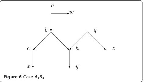
CaseA1B3. Assume that there is a normal path froma
to somew ÎX such that the path does not go through
b. Assumeb has one normal childc and a hybrid child
hfor which there is exactly one other parentq. There is a normal path from c tox Î X, from hto y Î X, and from q to z Î X. See Figure 6. Since Nis normal, an argument like that for Lemma 4.4 shows that Figure 6 is accurate for the situation.
In this situation, by Lemma 4.4(2), d(a,x;N) = [d(x,r;
N) +d(x,w;N)- d(r, w;N)]/2. In the equiprobable case, by Lemma 4.7, withb =q1,x1 =x,z =x2, d(b,x;N) =d (x, y; N) - d(r, y; N) + [d(r, x; N) + d(r, z; N) - d(x, z;
N)]/2.
Finallyω(a,b) =d(a,x;N)- d(b,x;N). In the non-equi-probable case, Lemma 4.9 witha=q3andb=q2yields the computation of w(a,b) =wq3,q2(N) and Lemma 4.9(i) showsa(b,h) =a(q2,h;N) = 1-a(q1,h;N).
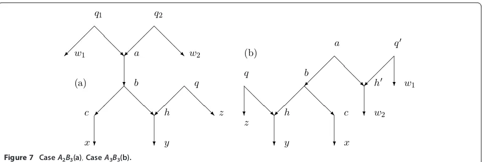
Case A2B3. Assume a is hybrid and b is its unique
child. Since a is hybrid it has two parents q1 and q2. Choose a normal path fromq1 tow1 Î X and from q2 to w2 Î X. Assume b has one normal child c and a hybrid childhfor which there is exactly one other par-entq. Choose a normal path fromctoxÎX, fromhto
yÎ X, and fromqtozÎ X.
See Figure 7a. An argument like that for Lemma 4.4 shows that the figure accurately represents what is needed in the argument. In particular, the normal paths
from q1 tow1, from q2 tow2, and from q toxhave no
vertex in common. Similarly the paths fromq toz, from
bto x, and fromhtoy have no vertex in common. By Lemma 4.4,d(a,x;N) = [d(x,w1;N) +d(x,w2;N) -d(w1,w2;N)]/2. In the equiprobable case, by Lemma 4.7,
d(b,x;N) =d(x,y; N)- d(r, y; N) + [d(r, x; N) +d(r,z;
N)- d(x,z;N)]/2.
In the non-equiprobable case, Lemma 4.9(ii) or 4.9(iii) similarly yieldsd(b,x; N). But ω(a,b) = d(a, x;N)- d(b,
x; N) since the path fromatox is normal, so subtract-ing these formulas leads to a formula forω(a,b).
CaseA3B3. Assume thata has a hybrid childh’with
other parentq’. Choose a normal path from q’ tow1Î
X and from h’ to w2 Î X. Assume b has one normal child cand a hybrid child hfor which there is exactly one other parentq. Choose is a normal path fromctox ÎX, fromhtoyÎ X, and fromqtoz ÎX.
See Figure 7b. The argument will make two uses of Lemma 4.7 or 4.9, and Figure 7b accurately represents the situation by arguments like those in Lemma 4.4.
In the equiprobable case, by Lemma 4.7,d(a,x;N) =d
(x, w2; N)-d(r, w2; N)+[d(r, x; N)+d(r, w1; N)-d(x, w1;
N)]/2,d(b,x;N) =d(x, y; N)- d(r, y;N) + [d(r, x; N) +
d(r,z; N)- d(x, z;N)]/2.
But then ω(a, b) = d(a, x; N) - d(b, x; N) since the path from ato xis normal. In the other case, Lemma 4.9(ii) or 4.9(iii) yields d(a, x; N) and d(b, x; N) and again ω(a, b) is determined. Moreover, Lemma 4.9(i) yieldsa(a,h’) anda(q,h).
Since all 9 cases yield a formula for ω(a, b) and also any relevant probability when ais parent to a hybrid
-? @
@ @ R
? ?
@ @
@ R
a w
b q
c
x
h
y
z
andb is a normal child ofa, the proof of the theorem is complete.
Corollary 4.11.Suppose N = (V, A, r, X) is a normal phylogenetic X-network such that each hybrid vertex has indegree 2 and, if it is not a leaf, outdegree 1. Let n= |
X|and a be the total number of arcs directed into any normal vertex. Then a≤n2.
Proof. We may assume that the arcs have weights and that each hybrid is equiprobable. Each of the weights
ω(u, v) if (u,v) is an arc directed into a normal vertexv
is uniquely determined from the n2
linear equations obtained from the n2 distances given by the tree-aver-age distance function. Hence there are at most n2 vari-ables.□
Figure 1 gives an example in whichn = 4 and there are exactly 42= 6 arcs directed into a normal vertex. Hence the bound in Corollary 4.11 is tight.
5 An example
We illustrate the calculations of Section 4 to find the values of the weight function given the network and the tree-average distance. Figure 4 exhibits a phyloge-netic X-network N = (V, A, r, X) with X = {1, 2, 3, 4, 5, 6, 7, 8, 9, 10, 11} and root 1 which satisfies the hypotheses of Theorem 4.1. Observe that by Corollary 3.4, N displays exactly 4 trees, and there are exactly four parent maps. Let ω be a weight function on A
such thatω(a,b) = 0 when b is hybrid butω(a, b)≥0 when b is normal. Let d(x, y) = d(x, y; N) denote the resulting tree-average distance between x and y in X. Suppose first that we assume equiprobability about the network, so each a(a,b) = 1/2 whenbis hybrid. There are 24 arcs for which we compute the weights as follows:
First, since 16 and 20 are hybrid, we haveω(17, 16) =
ω(15, 16) =ω(21, 20) =ω(23, 20) = 0. By Lemma 4.3(2),
ω(19, 8) = [d(8, 1) + d(7, 8)- d(1, 7)]/2,ω(19, 7) = [d
(7, 1) + d(7, 8)- d(1, 8)]/2, and we similarly findω(14, 3),ω(13, 2), andω(22, 10).
By Lemma 4.3(1),ω(1, 22) = [d(1, 9) +d(1, 11)- d(9, 11)]/2. By Lemma 4.3(3),ω(18, 19) = [d(1, 8) +d(6, 7) -d(1, 6)- d(7, 8)]/2,ω(12, 13) = [d(1, 2) + d(11, 3)- d(1, 11) - d(2, 3)]/2, and we similarly find ω(13, 14) and
ω(22, 12).
By Lemma 4.5, ω(20, 18) = [d(9, 8) + d(11, 6)- d(9, 11)- d(8, 6)]/2. By Lemma 4.4, ω(16, 5) = [d(5, 4) +d
(5, 6)- d(4, 6)]/2.
By Lemma 4.7 in the equiprobable case,ω(21, 9) =d
(9, 7) - d(1, 7) + [d(1, 9) + d(1, 11) - d(9, 11)]/2, ω(23, 11) = d(11, 7) - d(1, 7) + [d(1, 9) +d(1, 11) - d(9, 11)]/ 2, and we similarly findω(17, 6) andω(15, 4).
By Lemma 4.3(2),d(18, 6) = [d(6, 1) + d(6, 7) - d(1, 7)]/2. But thenω(18, 17) =d(18, 6) -ω(17, 6).
Similarly by Lemma 4.2(2)d(14, 4) = [d(4, 1) +d(4, 3)
- d(1, 3)]/2 and thenω(14, 15) =d(14, 4)-ω(15, 4). Similarly by Lemma 4.3(2)d(12, 11) = [d(11, 1) +d(11, 2)- d(1, 2)]/2 and thenω(12, 23) =d(12, 11)-ω(23, 11).
Finally, d(10, 9) is known since 10ÎX, soω(10, 21) =
d(10, 9) -ω(21, 9). This concludes the calculation of all the weights forNin the equiprobable case. Note that in several of these calculations, there were alternative choices possible. For example, we also haveω(22, 12) = [d(1, 4) +d(9, 11)- d(1, 9) - d(4, 11)]/2.
The general case where we do not assume equiprobabil-ity proceeds in a similar manner, different from the above only in the use of Lemma 4.9 in place of Lemma 4.7. We computeω(21, 9),ω(23, 11),a(21, 20), and a(23, 20) using Lemma 4.9 withx1= 9,x2= 11,x3= 2, andy= 7. We computeω(17, 6),ω(15, 4),a(17, 16), anda(15, 16) using Lemma 4.9 withx1= 6,x2= 4,x3= 3,y= 5.
6 Extensions
Theorem 4.1 applies only to normal phylogenetic net-works for which the indegree of each hybrid vertex is 2.
@ @
@ R
@ @
@ R
? @
@ @ R
@ @
@ R
? ?
w1
q1
a q2
w2
b q
c h z
x y
(a)
? @
@ @ R
? @
@ @ R
? @
@ @ R
? ?
a q
w1
h
w2
b
h
y
c
x q
z
(b)