Some New Aspects of Statistical Inference for Multistage Dose-Response Models with Applications

On the Occasion of his 75th Birthday Anniversary PJSOR, Vol. 8, No. 3, pages 441-478, July 2012

Some New Aspects of Statistical Inference for Multistage

Dose-Response Models with Applications

Bimal K. Sinha

Department of Mathematics & Statistics,

University of Maryland, Baltimore County, USA [email protected]

Leonid Kopylev

National Center for Environmental Assessment,i

Office of Research and Development,Environmental Protection Agency, USA [email protected]

John Fox

National Center for Environmental Assessment,ii

Office of Research and Development,Environmental Protection Agency, USA [email protected]

Abstract

Applications of the results to dose-response multistage models serve as illustrations. The paper considers various scenarios, and is expected to be of interest to practitioners of risk analysis.

Keywords: Benchmark dose, BMDL, Confidence limits, Dose-response models, Likelihood ratio tests, Maximum likelihood estimates, Multistage Weibull model, Parameters on the boundaries, Profile likelihood

1. Introduction

1.1 Dose-Response Models and Risk Estimates

Quantitative risk assessment for toxic and carcinogenic chemicals relies largely upon fitting dose-response models to data from animal bioassays. A variety of models are in use (Krewski and van Ryzin, 1980, Filipsson et al. 2003, U.S. EPA 2006) to represent both quantal (dichotomous) and continuous responses. Toxicological experience and principles indicate that the response will generally be bounded and non-decreasing (Eaton and Klaassen 2001).

conducted with mice or rats, typically in 3--5 dose groups including the control, each having 10--50 animals.

The maximum likelihood estimation for the parameters  employs the binomial likelihood





=0

( | ) = m i ( , ) 1x_i ( , )n xi _i

i i

i i

n

L x P d P d

x

    _  

   



(1)

The benchmark dose method (Crump 1984, Filipsson et al. 2003, Parham and Portier 2005) consists of estimating a lower confidence limit for the dose associated with a specified increase  in adverse response (i.e., increased risk) above the background level. In practice, the specified increase is typically 1% to 10% for cancer quantal response models (Filipssonet al. 2003, Parham and Portier 2005).

We will use "absolute risk" to refer to the probability P d( , ) modeled by a dose response model for a quantal response. The increase in risk above background for a quantal response is quantified as "extra risk" or "additional risk" (Filipsson et al. 2003). These quantities are defined below.

: = ( , )

Absolute Risk AR P d  (2)

: = ( , ) (0, )

Additional Risk ADR P d  P  (3)

( , ) (0, )

: =

1 (0, )

P d P Extra Risk ER

P

 





 (4)

The benchmark dose may be determined for any of these risk types. For example, the benchmark dose for extra risk of  is the solution of

( *, ) (0, )

( ) : *: =

1 (0, )

P d P

Benchmark Dose BMD d

P

 







 (5)

1.2 Statistical Inference

Statistical inference for chemical risk assessment has mainly emphasized finding confidence limits for the dose associated with a specified risk and for the risk associated with a specified dose. In this context, the profile likelihood method as applied in Crump and Howe (1985) and in U.S. EPA's Benchmark Dose Software (U.S. EPA 2006) assumes that 2log L( ( | )) x is distributed as 2

1

 . This is correct, asymptotically, under certain regularity conditions (Rao 1973, Cox and Hinkley 1974), one of which is that the true parameters are interior to the parameter space (for more details, see: Chernoff (1954), Feder (1968) and Self and Liang (1987); see also Molenberghs and Verbeke (2007) for a nice summary with applications). However, when one or more parameters (those of interest, or nuisance parameters, or both) lie on the boundary of the parameter space, the distribution of the likelihood ratio test statistic may not be 2

1

limits of model parameters are often approximated by Wald intervals, which are known to be inaccurate (Bailer and Smith 1994, Moerbeek et al. 2004, Nitcheva et al. 2007). These problems were acknowledged long ago (Crump et al. 1984), but have not been resolved clearly for the practitioners of dose-response modeling.

Research problems

Our primary goal in this paper is to develop appropriate asymptotic statistical methods in a very general multi-parameter framework when some parameters may lie on their boundaries. Our focus is mainly on the asymptotic properties of the MLEs and the LRTs. The problem of their actual computation, which involves use of sophisticated computer software and codes, is not discussed here. As an important application of the asymptotic theory, we discuss in detail inference about the parameters j in the multistage model (6) and about the quantities of interest, namely, AR, ADR, ER and BMD, when some of the basic parameters may lie on their boundaries. This is a significant point that has not been properly addressed in the relevant literature dealing with such models.

In the sequel, we discuss one commonly used model for quantal responses, called the multistage model:

=0

( , ) = 1 ( k j)

j j

P d  exp 



 d (6)

In applications, the coefficients 's are often constrained to be non-negative so that the dose-response function will be non-decreasing.

While AR, ADR and ER are direct and simple functions of , the benchmark dose d* (5) can obviously be a complicated function of , especially when k is large. To circumvent this potential difficulty, we proceed in an alternative fashion. Note that

*( ) = ( )

d    satisfies:

2

1 2

(1/ (1 )) = * * *k k

ln  d  d    d (7)

We propose to test H0 : ( ) =   versus H1 : ( )   for a given  > 0. If H0 is accepted, we include  in the confidence interval for  ( ). Otherwise, we exclude it.

We carry out this procedure for all possible values of  , thus hopefully generating an interval of accepted  -values, all belonging to the acceptance set, and thereby leading to the lower and upper bounds of  , which is ( ). Since ( ) is linear in , a test for

0

H versus H1 is easily carried out! In fact, since ln(1/ (1)) =   1  2 2   k k is

equivalent to 1

1 2

(1/ (1 )) / = k

k

ln _    _{  }    _{, we can work with a}

re-parametrization of the parameters 1

1 2 1 1 2 2

( , , , ) ( * = k , , , )

k k k

  _  _    _{  }     _ 

with 1* staying away from the boundary even if some of the 's may lie on their

boundaries.

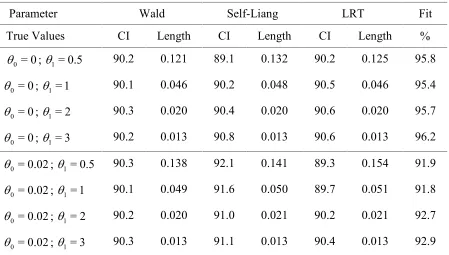
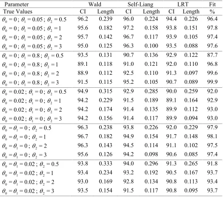
from a host of keypapers on this topic, notably from Self and Liang (1987). We develop both profile likelihood based inference (LRT) as well as Wald-type inference for a variety of situations with respect to boundary parameters. These results can be applied to a wide variety of models used in dose-response analysis. Applications to the specific multistage models (6) are discussed in Section 3. Simulations for linear, quadratic and cubic multistage models are reported in Section 4. These simulations clearly reveal that the use of Self & Liang's procedure over the Wald procedure considerably improves the expected lengths of the confidence intervals for all the relevant parameters. Some concluding remarks and directions for future research are mentioned in Section 5. An Appendix at the end contains a proof of a basic result of the paper.

2. New results on boundary value problems

Let us recall the general discussion mentioned in the previous section about the asymptotic properties of the MLEs in multi-parameter problems and the asymptotic distribution of the likelihood ratio test of a function of such parameters. Let X denote a random data set which is typically a collection of N independent and identically or independent but non-identically distributed random variables and let  = ( , , )1  p denote a p-dimensional real parameter vector which governs the distribution of X

through a joint density f X( | ) or equivalently the likelihood function L( | ) X . Let us assume that _{R}p _{and we write}

1

= _p

    where it is assumed that ii,

= 1, ,

i  p. We also assume that the p parameters 1, , p are functionally independent. Keeping the specific dose-response multistage Weibull models in mind, we further assume that i = [ , )i0  , a half-closed interval or i = ( , )i0  , an open interval,

where i0 is specified. In the former case, i0 is referred to as a boundary point of i, and in the latter case, all points of i are interior points. In most dose-response models,

0 = 0

i

 or 1 for all i. The statistical problem in such a set-up is to estimate the parameters  and test suitable hypotheses about  or some functions thereof based on the data set X . Since often the joint density or the likelihood function can be quite complicated as in the case of dose-response multistage Weibull models, both estimation of  and tests about  are carried out using suitable asymptotic theory under the assumption of a large sample size N .

LRTs unjustified and incorrect. Fortunately, this point has indeed been seriously addressed in the literature and a series of papers concerning this vital issue have appeared, most notably by Self and Liang (1987).

Based on Chernoff (1954), Feder (1968), Moran (1971), Chant (1974), Fahrmeir and Kaufman (1985), Self and Liang (1987), Geyer (1994), and Vu and Zhou (1997), the following two general results can be stated under fairly standard regularity conditions on the joint density of X and nature of . The conditions are typical Cramer-type and are satisfied in our applications to multistage dose-response models.

Let ˆN denote the MLE of  when the likelihood function L( | ) X is maximized wrt

 . Recalling the very general nature of , the maximization of the likelihood with respect to (wrt)  might mean unrestricted maximization in an open set (actually

product of open intervals) or a restricted maximization in a product of open and half-closed intervals, depending on which parameters can assume their boundary values. We will call these as natural restrictions on  and reserve the use of the term restricted

maximization to the situation when the components of  are restricted by a null hypothesis of the form H0: 0. Assume *= ( , , )1*  p* to be the true value of the vector parameter  and let _{I( )}* _{be the Fisher information matrix evaluated at  =} *_,

which is assumed to be positive definite with _{( ) = [ ( )]}* _{I }* 1_{. For ready reference, we}

also mention that the ( , )i j th element of the information matrix _{I( )}* _{is computed as} 2

[ ( | )]

i j

E lnL X

   

  where the expectation is evaluated at

*

 . It is understood that in

case of boundary points, the derivatives are computed from appropriate directions.

Our first result is concerned with the asymptotic distribution of the MLE ˆ_N of  under the true value _* _{where }* _{is either an interior point in  or a combination of both}

interior and boundary points of .

Proposition 2.1. The asymptotic distribution (as N _{) of the} p-vector

* *

1 1

ˆ ˆ

( N , , pN p)

N   _   is the same as the (exact) distribution of the MLE ˆ( )Z of  based on a normal p-vector Z with mean  and dispersion matrix _{( )}* _{under  = 0.}

Here the MLE ˆ( )Z of  based on Z is computed under the assumption that the mean vector  of Z lies either in an open set in _Rp _{including the point 0 , corresponding to}

the case when * *

1

( , , ) _p is an interior point in  with reference to the distribution of

X , or in a product of open and half-closed intervals of the type ( , ),[0, ) , whose nature depends on which true parameters *

i

 's are the boundary points i0's of  with

reference to the distribution of X . Thus, if * 0

=

i i

When in fact * 0

i i

  , the maximization of the normal pdf of Z is carried out wrt , taking i 0. Under these conditions, it is no longer true that Z is the MLE of  based on Z, and hence the asymptotic normality of ˆN does not hold! Moran (1971), Chant (1974) and, most importantly, Self and Liang (1987) have clearly spelled out the MLEs of  based on Z under various scenarios of boundary points. Once the MLEs of  based on Z are identified and their joint distribution under normality of Z is derived, this

would provide the asymptotic joint distribution of * *

1 1

ˆ ˆ

( _N , , _{pN p})

N   _  . Because of

the nature of  assumed above, it will hold that ˆiN i0, for all i. Thus, in the exact

and asymptotic distributions of ₍ˆ *₎

iN i

  _{, it will hold that this difference can assume}

both positive and negative values when *

i

 is an interior point of i = ( , )i0  , and is

nonnegative when * 0

=

i i

  , the boundary point of i = [ , )i0  .

One major goal of this paper is to further develop this part when we have one, two or three boundary points, clearly explaining the joint distribution of the resultant MLEs of 

based on Z which then readily yields the asymptotic joint distribution of the MLEs of 

under X . This knowledge is useful when one is interested in developing Wald-type inference about a smooth function of  based on the MLEs ˆN of.

To be specific, we establish the following results in Section 2 concerning the asymptotic distribution of the MLE ˆ_N of , which is computed by maximizing the likelihood function L( | ) X wrt  _.

 _{The asymptotic joint distribution of} * *

1 10 2 2

ˆ ˆ ˆ

( N , N , , pN p)

N     _   with one

boundary point * 1 = 10

  , 1 = [ , )10  , i*>i0, i = ( , )i0  , i2.

 _{The asymptotic joint distribution of} * *

1 10 2 20 3 3

ˆ ˆ ˆ ˆ

( N , N , N , , pN p)

N         

with two boundary points * 0

=

i i

  , i = [ , )i0  , i= 1, 2, *j >j0, j = ( , )j0  ,

3

j .

 _{The asymptotic joint distribution of}

* *

1 10 2 20 3 30 4 4

ˆ ˆ ˆ ˆ ˆ

( N , N , N , N , , pN p)

N         _  _{with three boundary points}

* 0

=

i i

  , i = [ , )i0  , i= 1, 2,3, *j >j0 , j = ( , )j0  , j4.

We now describe another important aspect of the papers by Moran (1971), Chant (1974), and Self and Liang (1987) in the context of the derivation and properties of the likelihood ratio tests for  based on X when some parameter points may lie on the boundary. To make matters simple and easy to understand, let us consider the following two testing problems about just one component, say 1, of .

Problem 2.1. Test the null hypothesis H₀: = _{1 10} versus H₁: ₁ ₁₀ where

> 0

 . Here naturally ₁ is an interior point of ₁.

Problem 2.2. Test the null hypothesis H0: = 1 10 versus H1: > 1 10 where 10 is the

boundary point of 1 = [ , )10  .

It is well known that when both , the general parameter space, and 0, the parameter

space under a null hypothesis, are smoothin the sense of being open sets in _Rp _{and in a} lower dimensional subspace, respectively, the asymptotic distribution of 2 (ln LRT)

under the null hypothesis is central chi-square with an appropriate df . However, this result is far from being true when some parameters may lie on the boundary either under the null hypothesis or even otherwise. It is precisely in the context that  and ₀ may not be open sets in _Rp _{that we have the following general result primarily due to Self and} Liang (1987). We remark that Self and Liang's results on the asymptotic distribution of the LRT are quite general, but here we state the results keeping in mind the two null hypotheses given above under Prob. 2.1 and Prob. 2.2.

Proposition 2.2.

(a) Consider the problem of testing the null hypothesis H0: = 1 10 versus

1: 1 10

H    , for some  > 0 when 1= ( , )10  , and suppose we compute the LRT

by maximizing L( | ) X wrt   and also under H0. Write

0 = { : = 1 10  , , ,2 p

  _ unspecified}. Then the null distribution of the profile log

likelihood based LRT using X , namely, the null distribution of

0 ( | )

2

( | )

max L X ln

max L X





 





 

  

 

  (8)

is asymptotically equivalent to the distribution of the profile log likelihood based LRT using Z under N[ , ]  , namely, the distribution of

* *

0 ( | ) ( | )

min_ Q  Z min_ Q  Z

   (9)

when  = 0. Here _{Q( | ) = ( Z Z) [ ] ( } 1 _{Z) is the exponent of the normal}

likelihood of Z with mean  and dispersion , minimum under * 0

generally, _* _{is a translation of  by} 0

 so that _* _{includes the point 0 in the}

parameter space of Z.

(b) Consider the problem of testing the null hypothesis H0: = 1 10 versus H1: > 1 10,

and suppose we compute the LRT by maximizing L( | ) X wrt   and also under

0

H . Write 0 = { : , , ,  10 2  p unspecified}. Then the null distribution of the profile log likelihood based LRT using X , namely, the null distribution of

0 ( | )

2

( | )

max L X ln

max L X





 





 

  

 

  (10)

is asymptotically equivalent to the distribution of the profile log likelihood based LRT using Z under N[ , ]  , namely, the distribution of

* *

0 ( | ) ( | )

min_ Q  Z min_ Q  Z

   (11)

when  = 0. Here, as before, _{Q( | ) = ( Z Z) [ ] ( } 1 _{Z) is the exponent of the}

normal likelihood of Z with mean  and dispersion , minimum under * 0

  is computed when 1= 0 and 2, ,p are unspecified in ( , )  , and minimum under

*

 is computed when ₁0 and all the other parameters  are unspecified in

( , )  . In other words, as before, _* _{is a translation of  by} 0

 so that _* _includes

the point 0 in the parameter space of Z.

Remark 2.1. It should be noted that the null hypotheses mentioned above are concerned only with 1 and do not mention anything about the nuisance parameters 2, , p. It is quite possible that some of the nuisance parameters may lie in a parameter space containing the boundary points. In other words, it is possible that ii = [ , )i0  for

> 1

i . When this happens, it is implied that the minimization wrt  in the quadratic form

( | )

Q Z is done under the restriction that _i0, implying that 0 is a boundary point wrt i

 rather than being an interior point.

Moran (1971), Chant (1974) and, most importantly, Self and Liang (1987) discussed at length computation of the LRT based on Z and its null distribution under various forms of the null hypothesis well beyond the two cases mentioned above. In general, as remarked earlier, it follows that the null distribution of the LRT based on Z is central chi-square when *

0

 consists of interior points of the mean vector  in the normal distribution of Z. However, this distribution is quite often a mixture of chi-squares when

* 0

 contains some boundary points of  as in Prob. 2.2 above.

A second major objective of this paper is to discuss in detail the null distribution of the LRT based on Z for testing the two hypotheses about 1 mentioned above under Prob.

Referring to Prop. 2.1, we should note that once the MLEs of  based on Z under _*

and their joint distribution are derived, we can use Prop. 2.1 to approximate the joint as well as the marginal distributions of the actual MLEs of  based on X . These distributions can then be effectively used to draw suitable Wald-type inference about a smooth function of  such as tests for a single component or a linear function of the components of , thus providing an alternative to the profile likelihood approach.

Likewise, referring to Prop. 2.2, once the LRT of H0 versus H1 based on Z is derived

and its null distribution is obtained, we can use it to get the approximate cut-off points of the LRT based on X . We remark that this reduction of the original inference problem based on X with an arbitrary distribution to a canonical form using Z which has a normal distribution, though only asymptotically valid, is a key feature of the asymptotic theory and the spirit of all the earlier works of these authors.

We are now in a position to describe the main results of this section. Based on the distributional assumption Z N_p[ , ]  , where  is unknown and  is positive definite known, we develop some new results for exact inference on 1 in presence of a few

nuisance parameters, allowing the possibility that some of the nuisance parameters may lie on the boundaries.

Towards deriving the LRT of H0: =1  versus H1:1 for some  > 0 based on Z,

which corresponds to testing H0: = 1 10 versus H1: 1  10 for some  > 0 in

the original distribution of X , we note that the likelihood function of Z, namely,

( | )

L  Z can be written as

1

( | ) = [ ( ) ( )].

L Z K exp Z_{ } _ Z_ ₍₁₂₎

Since we assume that the p parameters are functionally independent, for testing

0: =1

H   versus H1:1 based on Z, it is well known that if the parameter vector

 is an interior point in _Rp_{, which means the true parameter values of the parameter}

1



of interest as well as the nuisance parameters 2, , p are interior points, then the usual normal test based on Z1 is the LRT and it provides a a valid test. Recall that the

dispersion matrix of Z is assumed known which results in a normal test rather than a t -test.

As mentioned earlier, Self and Liang (1987), based on previous works of Chernoff (1954), Chant (1974), Moran (1971) and Shapiro (1985), developed appropriate solutions to this kind of problem for a wide variety of scenarios involving several parameters under

0

parameters in a typical multi-normal set-up can indeed lie on the boundary and also because of the fact that such situations often arise in applications.

Following essentially Self and Liang's ideas, we derive below the likelihood ratio tests (LRTs) of H0 versus H1 based on Z, allowing one, two and three nuisance parameters

to be on the boundary. It turns out that, as one can expect, the form of the LRT becomes quite complex with the increase in the number of nuisance parameters which lie on the boundary. In the sequel, we also derive the maximum likelihood estimates of all parameters  based on Z under the condition that some of the parameters may lie on the boundary, and derive their joint and marginal distributions. As mentioned before, these results would be useful when one is interested in deriving Wald-type asymptotic inference based on X about a smooth function of , and in particular, about a linear function of these parameters which is the case for dose-response multistage Weibull models mentioned in Section 1.

Some standard results from classical multivariate analysis which are needed in the sequel are listed below. Write Z = (Z Z(1), (2)),  = ( , (1) (2)) where Z(1):q1, Z(2): (p q ) 1,

(1):q 1

  , (2): (p q ) 1, and (11) =var Z( (1)), (22) =var Z( (2)), and (12) =cov Z Z( (1), (2))

 . Then:

distribution of a quadratic form

1 2

[Z] ( ) [   Z]p (13)

marginal distribution

1 q[ ,(1) (11)]

Z N   (14)

conditional distribution of Z₁, given Z₂ =z₂

1 1

1| 2 q[ 1 (12)( (22)) ( 2 2), (11) (12)( (22)) (21)]

Z z N  _{  }  z _ _{   }  _

 (15)

2.1 One parameter on the boundary

In this subsection we assume that there is one parameter, say i, which may lie on the boundary in the sense that ii = [ , )i₀  , and carry out appropriate inference about . Before we develop inferential tools, let us make a remark about testing for the existence of a boundary parameter.

Consider a general multi-parameter model based on X involving p parameters

1

= ( , , )_p

  _    where    = 1  p with i = [ , )i0  or ( , )i0  for all i.

Suppose it is suspected that one parameter lies on the boundary! How do we determine which one? Here is an ad hoc approach. Assuming that  i = i0 is the point on the

boundary, we can maximize the likelihood L( , ,1   i1, i1, , | =   p i i0, )X wrt 0

= ( , )

j j j

     for all j i and compute the maximum value of the likelihood, say i

L. Comparing L1, , Lp and selecting the index k such that Lk =max L( , , )1 Lp , we can conclude that k lies on the boundary. Alternatively, we can test the hypothesis

0i: =i i0

index k for which k is the smallest with the conclusion that k is likely to lie on the boundary. Details about such a test are given below.

Let us consider the two testing problems about 1 mentioned earlier, under the

assumption that there is one boundary parameter. We will derive exact tests based on Z

which would yield asymptotic tests based on X . Consider testing H0: =1  versus 1: 1

H   based on Z N[ , ]  . We distinguish between two cases depending on whether the parameter on the boundary is itself the parameter of interest (1) or a

nuisance parameter, say 2. In the former case, we take  = 0 as the boundary point of *

1 = [0, )

  and write H1: > 01 while the other parameters are free. In the latter case,

we take  > 0 as an interior point of *

1 = (0, )

  , and assume that one of the remaining unspecified nuisance parameters, say 2, may lie on the boundary in the sense that

2 [0, )

   . Note that, by definition, a nuisance parameter can never be known so that we cannot conclude that 2 = 0!

Case 2.1.1 ₁ is a boundary point. This has been discussed at length in Self and LiangError! Reference source not found.who derived the LRT of this problem. It turns out that the LRT is based on 2

1 [ > 0] /1 11

Z I Z  and its null distribution is a 50:50 mixture

of 2 0

 and 2 1

 distributions. Details are omitted.

Case 2.1.2 ₁ is an interior point and ₂ is a boundary point. To derive the LRT for

0: =1 10

H    versus H₁:  ₁  ₁₀ for some  > 0 on the basis of X , note that, asymptotically, this is equivalent to testing H₀: =₁  versus H₁:₁ for  > 0 based on Z. We proceed to apply Prop. 2.2. It is clear from the expression of the likelihood function L( | ) Z given in (12) that what matters is the quadratic form Q( | ) Z given by

1

( | ) = ( ) ( ).

Q Z Z_ _ Z_ ₍₁₆₎

Writing Q( | ) = ( , | , ) Z Q 1 2 Z Z1 2 Q Z( , ,3  Z Z Zp| , ; )1 2  where the first part is the

marginal bivariate quadratic of ( , )Z Z1 2 and the second part is the (p2)-dimensional

conditional quadratic of ( , , )Z3  Zp , given ( , )Z Z1 2 , it follows from Self and Liang

(1987) that due to the interior nature of the parameters 3, , p, the only part we need to study is the first part, and maximization of the likelihood corresponds to finding the two minimums of the first part, one under the union of null and alternative hypotheses, and the other under the null hypothesis.

To derive the maximum likelihood estimates (MLEs) of the parameters  under the union of null and alternative parameter spaces, we can express Q( , | , ) 1 2 Z Z1 2 as

1 2 1 2 2 2 1 2 1 2

( , | , ) = ( | ) ( | ; , )

Q  Z Z Q Z  Q Z Z   (17)

where Q Z( | )2 2 is the marginal pdf of Z2 and Q Z Z( | ; , )1 2  1 2 is the conditional pdf

interior nature of ₁, the minimum value of Q Z Z( | ; , )_{1 2}  _{1 2} wrt ₁ is 0 , irrespective of the value of ₂. Now a minimization of Q Z( | )₂ ₂ wrt ₂ subject to ₂ 0 readily yields:

2 2 2

2 2

2 22 2

( | ) = 0 > 0

0

= / 0.

min Q Z if Z

Z if Z

 





 (18)

To minimize Q( , | , ) 1 2 Z Z1 2 wrt2 under the null hypothesis when 1 = , we write

1 2 1 2 1 1 2 1 1 2

( , | , ) = ( | = ) ( | ; = , )

Q  Z Z Q Z   Q Z Z    (19)

where Q Z( | = )1 1  is the pdf of Z1 under the null hypothesis and Q Z Z( | ; = , )2 1 1  2

is the pdf of Z2, given Z1 when 1=. Since the first term is independent of 2, it is

clear that the minimum value of Q( , | , ) 1 2 Z Z1 2 wrt 2 arises essentially from

minimizing Q Z Z( | ; = , )2 1 1  2 wrt 2. Since

2 2

2 2 1

1

2 1 1 2 2

22

[ ( )]

( | ; = , ) =

(1 )

Z Z

Q Z Z

              (20)

minimization of Q Z Z( | ; = , )2 1 1  2 wrt2 under the condition 2 0 readily gives

2 1 1 2 2.1

2 2 2.1 2.1 2 22

[ ( | ; = , )] = 0 > 0

0

= 0

(1 )

min Q Z Z if Z

Z _{if Z}

         (21) where 2

2.1 2 1

1

= ( )

Z Z  Z 



  . Hence we get

2 1

1 2 1 2 2.1

1 2 ₁₁

2 2 2.1 1 2.1 2 11 22 ( )

( , | , ) = , > 0

= ; 0

( )

= , 0.

(1 )

Z

min Q Z Z if Z

Z

Z _{if Z}

      _        _{ }  (22)

Combining (18) and (22), and taking the difference, we get 2 (ln LRT) = (W say) as

2

1 11 2 2.1

2 2

1 11 2 22 2 2.1

2 2

1.2 11 2 2.1

2 2 2.1 1 2 2.1 2 11 22

= ( ) / , > 0, 0

= ( ) / / , 0, > 0

= / (1 ), 0, 0

( )

= , > 0, < 0.

(1 )

W Z if Z Z

Z Z if Z Z

Z if Z Z

Z

Z _{if Z Z}

                    _  (23)

It is easy to verify that when  = 0, W reduces to 2

1 11

To derive the null distribution of W for any given , we assume without loss of generality that 1 =2 = 1 and  = 0. It is proved in the Appendix that the cdf of W is

given by the following.

Theorem 2.1The cdf G w( ) ofW , for 0 < <w _{, is given by the sum of four parts:}

( )i First part = ₀



_ 2_1 2_



(0,1) (0,1)

r w w

N dx N dv



  



  

 

 

 

 

(24)

( )ii Second part = w (0,1) (0,1)

w w N dx N dv

  

 



 

 

 

 

(25)

( )iii _ 22_

0

2

/(1 1

Third part = _{ w  )} __  _ N(0,1)dx N_ (0,1)dv

 





(26)

( )iv  _{ }22

2

1 /(1

1

)

= (0,1) (0,1)

Fourth part  ____ N dx  _   N dx





 



 (27)

The above distribution can be used to get a cut-off point of the statistic 2 (ln LRT) which can then be used to carry out the LRT based on X . Quite surprisingly, our simulations indicate that the above distribution does notdepend on !

We now discuss the application of Wald-type test for testing H0 versus H1. Towards this

end, we note from Self and Liang (1987) that the MLEs of the parameters i when 2

may be on the boundary are given by the following. Define 2

.2 2

2

= i i

i i

Z Z  _ Z .

Theorem 2.2The MLE of i, i= 1,3, , p when2 is on the boundary is given by

2 .2 2

ˆ = [ > 0]i Z I Zi Z I Zi [ 0].

   (28)

The marginal distribution of the MLE of i, which depends on the correlation i2

between Zi and Z2, is given below. This would be useful if one is interested in drawing

suitable inference about just one parameter i.

Theorem 2.3 The pdf of the MLE ˆ =i Ui of i is given by

 

 





 





2 2

2 2

2

2 2

2 2

2 1

2 1

0 2 2

2 2

.

2 1 2 2 1

i i i ii i

i i

ii i x

x

u

i

ii i ii i

u

e e

f u dx

  



 

    

 

 _{ } 

 

 



  _

  _

 

 



 

 



(29)

the first part, we first write down the bivariate normal pdf of Z₂ and Zi, and then integrate out Z₂ over (0, ) . The pdf of Ui for the first part is then directly obtained from the cdf of the first part upon differentiation wrt ui. This completes the proof.

Remark 2.2 Specializing to the case of testing H0: =1   10 versus H1: >1   10

based on X , we can easily derive a Wald-type test based on the MLE of ₁, namely, ˆ1N which is the standard MLE of  based on X under   with ₂ = [ , )₂₀  and

0

= ( , ) i i

  for i2. Because of the nature of H₀ and H₁, it makes sense to reject H₀

for large values of ˆ1N, i.e., when ˆ >1N cN for some cN. To determine the value of cN for a given level of significance , it follows that, asymptotically,

1 0 1 10 10 1 2 1.2 2

ˆ ˆ

= [P N >c HN| ] = [P N( N ) > N c( N )] P Z I Z[ ( > 0) Z I Z( 0) > N c( N )]

             .

We can now use the result of Theorem 2.3 to claim: N c( N ) =z | where z | is the

upper  cut-off point of the distribution of Z I Z₁ [ > 0]₂ Z I Z_1.2 [ ₂ 0] given in Theorem 2.3 for i= 1. Hence we reject H₀ when ˆ >₁N   ₁₀z _| / N . This is of course a very easy test to carry out without the need to compute a profile likelihood which is the basis of LRT. However, we should also note that we have taken a one-sided alternative as H1.

For a both-sided alternative, we may choose to reject H0 for large values of

1 10

ˆ

| N    | and determine the cut-off point appropriately. Note that this would provide an alternative approach to the profile likelihood method (LRT).

Remark 2.3 If one is interested in making inference about a linear combination of i's which excludes the boundary point ₂, we note that the distribution of

2 .2 2

2 2 2

= _i i i = [ _i i i] [ > 0] [ _i i i ] [ 0]

U



_cU



_c Z I Z 



_c Z I Z  is again readily obtained as the sum of two parts of which the second part (when Z2 0) is normal with mean 0 and

variance obtained from the variances and covariances of the residuals Zi.2's, and the other

part is a convolution of two normals. The latter term is obtained by writing down the bivariate normal pdf of (



_i₂c Zi i) and Z2, and then integrating out Z2 over (0, ) .

Thus, defining *

1 3

= ( ,0, ,.., )_p

c c c c , _2_{* = * *c c ,} *

2 2

= _i ci i i





_   and

2 2 2

2 2 2

2 2

= _ic_i_ii(1 _i ) _{i j }c c_{i j i}  _j( _ij  _{i j} )





 



 , the pdf of U is given by

( ) = ( )I II( )

f u f u  f u where

2 2

-2

2 2

( ) = I

u

e f u



2 * 2

2* *

2*

* 2*

0

2 2(1 )

( ) = /[2 1 ]

x

II

u xu

f u e dx



 



 





 _{ } 

 

 _ 

 

  _



(30)

Let us recall that the distribution of U given here is precisely the asymptotic distribution of N[



_i2c_{i iN}ˆ 



_i2c_{i i} ] and hence can be readily used for drawing valid asymptotic inference about



_i₂ci i . Note that this so-called Wald-type approach avoids computing profile likelihoods for testing hypotheses about [



_i₂ci i ].

Remark 2.4 If, on the other hand, we are interested in making inference about a linear function of the i's which also includes 2, naturally we need to derive the distribution of

2 2

2 ˆ ˆ

= _{i i i}

V



_c c . Since ˆ =2 Z I Z2 [ > 0]2 , it follows from (28) that the distribution of

V will again consist of two parts: one part, corresponding to Z2 < 0, is just normal and is

independent of Z₂. This is in fact the distribution of



_i2c Z_{i i.2}. The other part, for

2 > 0

Z , is obtained by first deriving the conditional distribution of



_i₂c Zi i which is normal and then convoluting it with c Z2 2. This argument leads to the pdf of V as

*

( ) = ( )_{I II}( )

f v f v  f v where ( )f vI is the same as f uI( ) , and f vII*( ) is given by

 

2

2 ₂

=1 (

2 *

0

)

2 2

( ) = .

2 p

i i i i

II

c

x e

f v dx

v x

 



  

  

  

  

 

 

 

 









(31)

We recall that the distribution of V given here is precisely the asymptotic distribution of

=1 ˆ =1

[ _ip i iN _ip i i]

N



c 



c and hence can be readily used for drawing valid asymptotic inference about



_ip₌₁ci i . Again, this approach avoids the computation of a profile likelihood.

2.2 Two parameters on the boundaries

We now discuss the case of two boundary parameter points. Kopylev and Sinha (2011) discussed the case when the parameter of interest and a nuisance parameter lie on the boundary. Here we consider the case when two nuisance paramaters lie on the boundary and the parameter of interest is an interior point.

Assume without any loss of generality that 2 and 3 lie on the boundary and our

consider both LRT and Wald-type tests for H₀: = _{1 10} versus H₁: ₁  ₁₀ for some  > 0 based on X .

As before, write Q Z( | ) = ( , , | , , ) Q Z Z Z_{1 2 3}   _{1 2 3} Q Z( , ,_{4 } Z Z Z Z_p| , , ; )_{1 2 3}  and recall that in the -space for Z, 2[0, ) , 3[0, ) and i  ( , ) for i2,3. Hence, for LRT as well as for Wald, we need to concentrate only on the first part. For the unrestricted MLEs of2 and 3, we get from Self and Liang (1987):

2 3 2 3 2 3

2.3 2.3 3

3.2 2 3.2

2.3 3.2

ˆ ˆ

( , ) = ( , ) , > 0, 0

= ( ,0) , 0, 0

= (0, ) , 0, > 0 = (0,0) , < 0, < 0.

Z Z if Z Z

Z if Z Z

Z if Z Z

if Z Z

    

    



(32)

Since the minimum of Q Z Z Z( | , ; , , )1 2 3   1 2 3 wrt 1 for any given ( , ) 2 3 is 0 and also

the minimum of Q Z( , ,4  Z Z Z Zp| , , ; )1 2 3  wrt 4, , p for any given 1, 2 and 3 is

0 , we get

* ( | ) = ( , | , )2 3 ˆ ˆ2 3

min_Q Z  Q Z Z   (33)

It is easy to show that the above minimum simplifies to

* 2 3

2

3 33 3 2.3

2

2 22 2 3.2

2 3 2 3 2.3 3.2

( | ) = 0, > 0, 0

= / , < 0, > 0

= / , 0, > 0

= ( , | = = 0), 0, 0

min Q Z if Z Z

Z if Z Z

Z if Z Z

Q Z Z if Z Z

 

 

 

 



 

(34)

Once ˆ2 andˆ3 are derived, the MLEs of the rest of the (interior) parameters are readily

obtained from Q Z Z( , , ,1 4  Z Z Zp | , ; )2 3  as the residualsof Zi, given ( , )Z Z2 3 , and are

given by

2 2 3 3

ˆ_{i =Z E Z Zi [ |i} ˆ _,Z ˆ_].

    (35)

To derive the LRT of H0: =1  versus H1:1  based on Z, we need to derive the

restricted MLEs of's under the null hypothesis H0. Without any loss of generality, let

us assume  = 0, and write

1 2 3 1 2 3 1 2 3 1 1 2 3

( , , | = 0, , ) = ( | = 0) ( , | ; = 0, , )

Q Z Z Z    Q Z  Q Z Z Z    . Since the first part is independent of 2 and 3, writing Y2 =Z2.1 and Y3 =Z3.1, we get from Self and Liang

2 3 2 3 2 3

2.3 2.3 3

3.2 2 3.2

2.3 3.2

ˆ ˆ

( , ) ' = ( , ) , > 0, 0

= ( ,0) , 0, 0

= (0, ) , 0, > 0 = (0,0) , < 0, < 0.

null Y Y if Y Y

Y if Y Y

Y if Y Y

if Y Y

   

  

 



(36)

Since as before the contribution from the minimization of Q Z( 4,Z Z Z Zp | , , ; )1 2 3  with

respect to 4, , p is 0 even under H0 due to the interior nature of the parameters 4, , p

 _  , it follows that

* 0 1 1

0

2 3 1 1 2 3

2 3

1 1 2 3 1 2 3

2

1 11 2.1 3.1

2

2 1.3

3 33 2 3.1 2.13

11 13

2

2 1.2

2 22 2

11 12

( | ; ) = ( | = 0)

( , | , = 0, , ) , 0

ˆ ˆ

= ( | = 0) ( , | , , )

= / , > 0, 0

= / , < 0, > 0

(1 )

= / ,

(1 )

min Q Z H Q Z

min Q Z Z Z

Q Z Q Z Z Z null null

Z if Z Z

Z

Z if Z Z

Z

Z if





 

  



  





 



 



 _ 

 

 

 2.1 3.12

2 1

1 11 2.1 2 3.1 3 2.1 2 3.1 3

2.13 3.12

0, > 0

= / ( / , / ) ( / , / ) ,

0, 0

Z Z

Z Z Z A Z Z

if Z Z

     



 

 

(37)

where the matrix A: 2 2 _{is defined as}

2

12 23 12 13

2

23 12 13 13

(1 )

= .

1

A    

   

   

 _{ } 

  (38)

Combining (34) and (37), the LRT of H₀: = 0₁ is obtained as W given by

* 0 *

0

= ( | ; ) ( | ).

W min_ Q Z  H min_ Q Z 

   (39)

To simulate the null distribution of W, we can take without any loss of generality

*

1 2 3

( , , )Z Z Z N[(0,0,0), ] where _* _{has its diagonal elements as 1. Upon generating}

the jth iteration element as ( ,Z Z Z1j 2j, 3j), we compute

2.3 3.2 3.1 2.1 2.13 3.12

(Z _j,Z _j,Z _j,Z _j,Z _j,Z _j), leading to a value wj ofW .

Obviously, the LRT of H₀ versus H₁ rejects H₀ when W computed as above is large. Again, quite surprisingly, it turns out from our simulation studies that the null distribution of W does not depend on the correlations between Z1 and ( , )Z Z2 3 .

For Wald-type inference about 1, we concentrate on the distribution of the MLE of 1

be obtained from (34) by conditioning on four disjoint subsets in ( , )z z_{2 3} -plane and deriving each component distribution and mixing them with suitable proportions. Details are omitted as this is similar to Theorem 2.1. This distribution can be used for testing

0: =1 10

H    based on X . Thus, if the alternative is H1: >1   10, a reasonable test

is to reject H0 for large values of the MLE ˆ1N of 1, namely, when (ˆ1N   10) >cN. To determine the value of cN for a given significance level , we can use the asymptotic null distribution of N(ˆ1N   10) in presence of two boundary parameters, which is

precisely the distribution mentioned above.

On the other hand, for a both-sided alternative H1:  1  10, a reasonable test is to

reject H0 for large values of |ˆ1N   10|. To determine the cut-off point for a given

significance level , we can again use the asymptotic null distribution of

1 10

ˆ

( N )

N     in presence of two boundary parameters, which is precisely the distribution mentioned above. Details are omitted.

Remark 2.5 Suppose we are interested in making a Wald-type inference about a linear function of , say



_i2,3c_{i i} which excludes the two boundary points 2 and 3.

Naturally we would then consider the distribution of



_i_2,3ci iNˆ . From (32), such a distribution can be obtained by conditioning on values of ( , )z z2 3 and then suitable

unconditioning.

Remark 2.6Suppose now that we are interested in making a Wald-type inference about a linear function of , say



_i_2,3ci i c2 2 which contains one of the boundary points, say

2

 . We would then consider the obvious statistic



i_2,3ci iNˆ c2 2ˆN. Its asymptotic distribution can be derived from the results given above.

Remark 2.7 Let us also assume that we are interested in drawing suitable Wald-type inference about a linear function of , which includes both the boundary parameters. Obviously, such a linear function can be written as =



_ici i and inference about  is drawn by studying the asymptotic distribution of W =



_ic_{i iN}ˆ . This distribution can also be derived from the above results.

2.3 Three points on the boundaries

In this section we deal with the case when three parameters lie on their boundaries. Kopylev and Sinha(2011) discussed the case when the parameter of interest and two nuisance parameters lie on the boundary. We consider here the case when all three nuisance parameters lie on the boundary and the parameter of interest is an interior point. Without any loss of generality, suppose 1, 2 and 3 are the three boundary parameters

interest. The relevant testing problem about ₄ is then to decide between

0: =4 40

H    versus H₁:₄ ₄₀ on the basis of X where  > 0 is specified. Equivalently (and asymptotically), this is the same as testing H₀: =₄  versus

1: 4

H   based on ZN[ , ]  , wheni 0, i= 1, 2, 3 and <j < for j> 3. To derive the LRT for the above testing problem, we proceed in the usual fashion by deriving both unrestricted and restricted (under H₀) MLEs of  based on X and computing the value of W = 2 ( ln LRT X( )), which is indeed the profile likelihood approach. To carry out the LRT test, naturally we need to determine the cut-off point of the null distribution of W. Following Self and Liang (1987) and Prop. 2.2, asymptotically, such a distribution is given by the distribution of the difference of two quadratic forms based on Z. This is discussed in Kopylev and Sinha (2011) and we have the following expressions for the unrestricted MLEs of the parameters  in the distribution of Z.

1 2 3 1 2 3 1 2 3

2.1 3.1 1 2.1 3.1

1.2 3.2 2 1.2 3.2

1.3 2.3 3 1.3 2.3

3.12 1.2 2.1 3.12

2.

ˆ ˆ ˆ

( , , ) = ( , , ) , 0, 0, 0 = (0, , ) , < 0, > 0, 0 = ( ,0, ) , < 0, > 0, 0 = ( , ,0) , < 0, 0, 0 = (0,0, ) , 0, 0, > 0 = (0,

Z Z Z if Z Z Z

Z Z if Z Z Z

Z Z if Z Z Z

Z Z if Z Z Z

Z if Z Z Z

Z

       

 

 

  

  

13 1.3 3.1 2.13

1.23 2.3 3.2 1.23

1.23 2.13 3.12

,0) , < 0, < 0, > 0 = ( ,0,0) , < 0, < 0, > 0 = (0,0,0) , 0, 0, 0.

if Z Z Z

Z if Z Z Z

if Z Z Z

 

   

(40)

where Z.. are the usual residual terms. Naturally we need to plug in these estimates of the MLEs in Q Z Z Z( , , | , , )1 2 3   1 2 3 and simplify to get an expression of the unrestricted

minimum, i.e., Q Z1( ). Writing Q Z( | ) = ( , , | , , ) Q Z Z Z1 2 3   1 2 3 Q Z( , ,4  Zp| ) , since the unrestricted minimum of the second term is 0 , it follows that

* 1 2 3 1 2 3

1 2 3

1 2 3 1 2 3

( | ) = _{0, 0, 0} ( , , | , , )

ˆ ˆ ˆ

= ( , , | N, N, N).

min Q Z min Q Z Z Z

Q Z Z Z



      

  

   

(41)

Because of the nature of ( ,  ˆ ˆ1N 2N, ˆ3N) given above in (40), it is obvious that the unrestricted minimum value of the relevant quadratic of the likelihood based on Z can be divided into eight disjoint sets, each set having a distinct value of the quadratic. This is explicitly presented in Kopylev and Sinha (2011).

On the other hand, to compute the restricted maximum likelihood under the null hypothesis H0: =4 40 in the X space which is equivalent to 4 = in the Z

space, note that all we need to compute are the restricted MLEs of 1, 2 and 3, subject

1 2 3 4 1 2 3 4

4 1 2 3 4 1 2 3 4

( , , , | , , , = )

= ( | ) ( , , | , , , , = )

Q Z Z Z Z

Q Z Q Z Z Z Z

    

       (42)

and note from (15) that the second quadratic can be expressed as

1

1 2 3 4 1 2 3 4 1.4 2.4 3.4 1.4 2.4 3.4

( , , | , , , , = ) = ( , , ) ( , , )

Q Z Z Z Z      Z Z Z _ Z Z Z _{ (43)}

where the residuals Z Z Z1.4, 2.4, 3.4 and  are defined as

.4 4 4 4

11 12 21 44

11 12 13

11 21 22 23

31 32 33

12 14 24 34

= ( ) / , = 1, 2, 3

= /

:3 3 =

. = ( , , )

i i i i i

Z Z    Z   i

                           _{ }        (44)

To determine the restricted MLEs of the parameters   1, ,2 3 which must be

non-negative, by minimizing Q Z Z Z Z( , , | , , , , = )1 2 3 4    1 2 3 4  , under the null hypothesis: 4 =

  , we can readily apply the above results. Based on the first step residuals

* * *

1.4 1 2.4 2 3.4 3

(Z = ,Z Z = ,Z Z =Z ) and their dispersion matrix  , we define the second step

residuals * * * * * * * * *

2.1 1.2 2.3 3.2 1.3 3.1 2.13 1.23 3.12

(Z Z Z Z Z Z Z Z Z, , , ) in the usual fashion. Then, the restricted

MLEs are given by:

* * * * * *

1 2 3 1 2 3 1 2 3

* * * * *

2.1 3.1 1 2.1 3.1

* * * * *

1.2 3.2 2 1.2 3.2

* * * * *

1.3 2.3 3 1.3 2.3

*

3.12 1.2

ˆ ˆ ˆ

( , , ) ' = ( , , ) , 0, 0, 0

= (0, , ) , < 0, > 0, 0

= ( ,0, ) , < 0, > 0, 0

= ( , ,0) , < 0, 0, 0

= (0,0, ) ,

N N N null Z Z Z if Z Z Z

Z Z if Z Z Z

Z Z if Z Z Z

Z Z if Z Z Z

Z if Z

               * * * 2.1 3.12 * * * *

2.13 1.3 3.1 2.13

* * * *

1.23 2.3 3.2 1.23

* * *

1.23 2.13 3.12

0, 0, > 0

= (0, ,0) , < 0, < 0, > 0

= ( ,0,0) , < 0, < 0, > 0

= (0,0,0) , 0, 0, 0.

Z Z

Z if Z Z Z

Z if Z Z Z

if Z Z Z

  



   

(45)

This then results in the restricted quadratic form

*

* 0

0

* 1 2 3 4 1 2 3 4

0

4 1 2 3 4 1; 2; 3; 4

( | )

= ( , , , | , , , = )

ˆ ˆ ˆ

= ( | ) ( , , | , null, null, null, = )

min Q Z

min Q Z Z Z Z Q Z Q Z Z Z Z

                  (46)

Using (41) and (46), we obtain the difference ( )Z between the two quadratic forms, whose distribution under ZN[0, ] is essentially the asymptotic null distribution of

2 (ln LRT)

nature of correlations among the estimates of the four parameters - one parameter of interest, namely, 4, and the three boundary parameters,   1, ,2 3. It may be remarked

that the null distribution of ( )Z may have to be obtained by simulation and it is obvious that we can take the dispersion matrix of Z as the correlation matrix, without any loss of generality. It would be interesting to check through simulations if this null distribution really depends on the correlations. Let us recall that this was not the case in the previous two instances.

A Wald-type test of H0: =4 40 versus the one-sided alternative H1: >4 40

based on X can be easily derived using the unrestricted MLE ˆ_4N of 4. This readily

follows from the conditional distribution of Z4, given ( , , )Z Z Z1 2 3 , and plugging in the

restrictedMLEs of   1, ,2 3 derived above. Such a test would reject H0 for large values

of ˆ4N, or N(ˆ4N40) and the cut-off point of its null distribution is

asymptotically computed from the distribution of the MLE of 4 based on Z in

presence of three boundary parameters. Similarly, for testing H0 versus the both-sided

alternative H1:4 40 , one could reject H0 for large values of N |ˆ4N 40 |

and the cut-off point is determined analogously from its null distribution. Obviously, this distribution, which depends on the correlation structure between Z4 and ( , , )Z Z Z1 2 3 , can

be easily derived.

3. Applications of general theory to multistage Weibull models

In this section we consider some applications of the general theory developed in Section 2 in the context of multistage Weibull models and analyze some relevant data sets. In the sequel, we consider three cases: linear Weibull model,