www.the-cryosphere.net/6/743/2012/ doi:10.5194/tc-6-743-2012
© Author(s) 2012. CC Attribution 3.0 License.
The Cryosphere
Refreezing on the Greenland ice sheet: a comparison of
parameterizations
C. H. Reijmer1, M. R. van den Broeke1, X. Fettweis2, J. Ettema1,*, and L. B. Stap1 1Institute for Marine and Atmospheric Research Utrecht, Utrecht University, Utrecht, The Netherlands
2D´epartement de G´eographie, Universit´e de Li`ege, Li`ege, Belgium
*now at: Faculty of Geo-Information and Earth Observations, University of Twente, Enschede, The Netherlands
Correspondence to: C. H. Reijmer ([email protected])
Received: 6 September 2011 – Published in The Cryosphere Discuss.: 18 October 2011 Revised: 1 June 2012 – Accepted: 4 June 2012 – Published: 11 July 2012
Abstract. Retention and refreezing of meltwater are
ac-knowledged to be important processes for the mass bud-get of polar glaciers and ice sheets. Several parameteriza-tions of these processes exist for use in energy and mass balance models. Due to a lack of direct observations, val-idation of these parameterizations is difficult. In this study we compare a set of 6 refreezing parameterizations against output of two Regional Climate Models (RCMs) coupled to an energy balance snow model, the Regional Atmospheric Climate Model (RACMO2) and the Mod`ele Atmosph´erique R´egional (MAR), applied to the Greenland ice sheet. In both RCMs, refreezing is explicitly calculated in a snow model that calculates vertical profiles of temperature, den-sity and liquid water content. Between RACMO2 and MAR, the ice sheet-integrated amount of refreezing differs by only 4.9 mm w.e yr−1(4.5 %), and the temporal and spatial vari-ability are very similar. For consistency, the parameteriza-tions are forced with output (surface temperature, precipi-tation and melt) of the RCMs. For the ice sheet-integrated amount of refreezing and its inter-annual variations, all pa-rameterizations give similar results, especially after some tuning. However, the spatial distributions differ significantly and the spatial correspondence between the RCMs is bet-ter than with any of the paramebet-terizations. Results are es-pecially sensitive to the choice of the depth of the thermally active layer, which determines the cold content of the snow in most parameterizations. These results are independent of which RCM is used to force the parameterizations.
1 Introduction
The surface mass balance (SMB) of a glacier is defined as the sum of all processes adding mass to the surface (accumu-lation) minus all processes removing mass (ab(accumu-lation): SMB=
Z
1 yr
dt (C+RF−SUs−SUds−ERds−RU) . (1)
The most important contribution to accumulation is snow-fall (C), with additional contributions of condensation and freezing of rainfall (RF). Removal of mass occurs by means of surface sublimation (SUs), sublimation of drifting snow (SUds), erosion by drifting snow (ERds), and melt and sub-sequent runoff (RU). Especially in the (sub)polar regions, where glaciers are usually polythermal, part of the meltwater percolates into the snow/firn and refreezes. Refreezing has been addressed by several authors, especially in relation to the estimated contribution of glaciers to sea level rise (e.g. Trabant and Mayo, 1985; Pfeffer et al., 1990, 1991; Braith-waite et al., 1994; Schneider and Jansson, 2004; Reijmer and Hock, 2008; Fausto et al., 2009). Although its importance for the Greenland Ice Sheet (GrIS) is acknowledged, refreezing estimates are scarce and cover a wide range of values (Box et al., 2006; Fettweis, 2007; Hanna et al., 2008; Ettema et al., 2009).
firn. The former can be split into homogeneous and het-erogenous infiltration of water and subsequent refreezing. In homogeneous infiltration water moves homogeneously from the surface through the snow and firn while in heterogeneous infiltration water infiltrates the firn along “pipes”, transport-ing water to larger depths (Marsh and Woo, 1984; Pfeffer and Humphrey, 1996). Refreezing is an important process: it increases the temperature and density of the snow/firn and delays and reduces runoff, it reduces melt in the ablation zone since it delays bare ice exposure, and impacts mass bal-ance profiles since it enhbal-ances mass accumulation around the equilibrium line and in the percolation zone above.
Most published work on refreezing describes homoge-neous infiltration and subsequent refreezing, and refers to es-timates for the GrIS, e.g. Pfeffer et al. (1991); Braithwaite et al. (1994); Fausto et al. (2009), although some estimates for individual glaciers in the Arctic are available (Trabant and Mayo, 1985; Schneider and Jansson, 2004; Reijmer and Hock, 2008; Wright et al., 2007). Bøggild (2007) and Wright et al. (2007) focussed on estimating superimposed ice for-mation, while Schneider and Jansson (2004) and Reijmer and Hock (2008) discussed the impact of refreezing on the glacier mass balance. A few observational studies on water infiltration are available as well (Marsh and Woo, 1984; Pf-effer and Humphrey, 1996; Humphrey et al., 2012). These observational studies show the importance of heterogeneous infiltration (piping) in the process of water infiltration and heating of cold firn. Given the wide range of applications and parameterizations, several authors attempted to compare the available parameterizations, most notably Janssens and Huy-brechts (2000) and Wright et al. (2007). These comparisons are hampered by the scarcity of refreezing observations, al-though Wright et al. (2007) did compare their results with observed superimposed ice layers in ice cores.
Janssens and Huybrechts (2000) studied the spatial vari-ability of refreezing in Greenland using different parameter-izations forced by output of a degree day model, and a tem-perature and precipitation climatology. They report a strong dependency on the chosen depth of the thermally active layer, which in these expressions largely determines the cold tent of the snow before the melting season starts. They con-clude that to account for the effects of refreezing below this depth requires a more comprehensive calculation of the tem-perature profile in the upper ice and snow layers. Several authors have explicitly incorporated the refreezing process in their energy, mass balance or (regional) climate models (Bougamont et al., 2005; Fettweis et al., 2005; Reijmer and Hock, 2008; Ettema et al., 2010b). For many climate stud-ies involving ice sheet evolution over centurstud-ies to millennia it is, however, still too computationally expensive to explic-itly include this process, and parameterizations will remain necessary.
This study aims at improving our insight in the perfor-mance of various refreezing parameterizations building on the study by Janssens and Huybrechts (2000). In the
ab-sence of observations, we use, as a reference, data of two re-gional climate models (RCMs) (Fettweis et al., 2005; Ettema et al., 2009) in which refreezing is explicitly calculated: the Regional Atmospheric Climate Model (RACMO2) and the Mod`ele Atmosph´erique R´egional (MAR). For consistency atmospheric data (temperature, precipitation, melt) from the RCMs are used to force the selected refreezing parameteriza-tions. We then compare the results of the parameterizations to the amount of refreezing calculated by the models, using RACMO2 as reference. We furthermore discuss the impact and sensitivity of the values of the different input parameters to the parameterizations.
2 Parameterizations
The amount of refreezing is limited by (1) the available energy, (2) the available pore space in the snow/firn, and (3) the available amount of water from melt, condensation, and rain. Following Janssens and Huybrechts (2000), we de-finePras the potential retention mass, which is the maximum amount of water that can be refrozen, and is determined by (1) and (2). We defineWras the available water mass (3) and Eras the effective retention mass, which is the actual mass refrozen in the snow.Pr,WrandErare related by:
Er=min[Pr, Wr] (2)
By defining the retention mass as outlined above it equals the amount of refrozen mass. On an annual time scale, this esti-mate includes the meltwater that refreezes in the cold snow in spring, the meltwater that refreezes at depth to form superim-posed ice and the capillary retained water that remains in the snow pack until the end of the melt season, and subsequently refreezes in winter. Note that the meltwater that refreezes in spring and superimposed ice may melt again and run off later in the melt season.
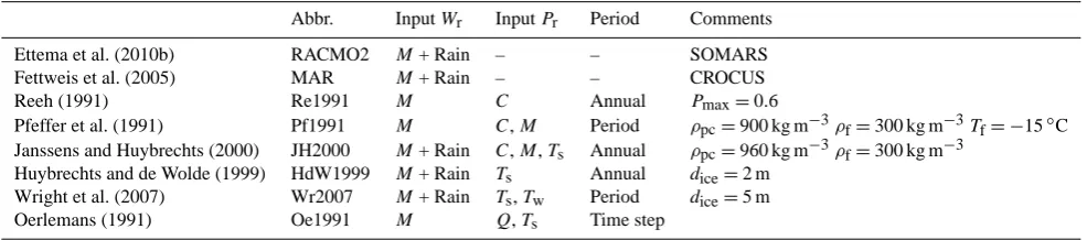
Below we describe several published parameterizations to calculatePrandEr, and the modifications we made where necessary. These methods do not necessarily include all im-portant processes or, for instance, include rain in the esti-mation ofWrand thusEr. Note that none of these parame-terizations include the process of heterogeneous infiltration. Table 1 presents the selected parameterizations and their re-quired input fields. The fields used to force the parameteri-zations are described in Sect. 3. All parameters referring to mass are in mm water equivalent (w.e.) unless stated other-wise.
2.1 Pmaxformulations
Pmaxformulations are the simplest way to calculate refreez-ing. They assume runoff to occur when the amount of re-freezing exceeds a maximum fraction (Pmax) of the annual snowfall (C):
Table 1. The tested parameterizations.Wrrefers to whether the available water mass in Eq. (2) equals melt (M) or melt plus rain. Input Prlists the input fields toPr, period refers to the period over which the input fields toPrare averaged. The constants presented in the last column are chosen to correspond to the settings in the original publications. Note that RACMO2 fields are used as input and reference unless stated otherwise.
Abbr. InputWr InputPr Period Comments
Ettema et al. (2010b) RACMO2 M+ Rain – – SOMARS
Fettweis et al. (2005) MAR M+ Rain – – CROCUS
Reeh (1991) Re1991 M C Annual Pmax=0.6
Pfeffer et al. (1991) Pf1991 M C,M Period ρpc=900 kg m−3ρf=300 kg m−3Tf= −15◦C Janssens and Huybrechts (2000) JH2000 M+ Rain C,M,Ts Annual ρpc=960 kg m−3ρf=300 kg m−3
Huybrechts and de Wolde (1999) HdW1999 M+ Rain Ts Annual dice=2 m Wright et al. (2007) Wr2007 M+ Rain Ts,Tw Period dice=5 m
Oerlemans (1991) Oe1991 M Q,Ts Time step
wherePris the potential retention mass. Reeh (1991) used Pmax=0.6, so that his modelled amount of melt from the GrIS agreed with other published estimates. Later research supports this value (Braithwaite et al., 1994).Pmaxmay be varied from 0, which is the lower bound with no refreezing possible, to 1, which represents a case in which all water may be refrozen. The latter is only a meaningful solution at the higher parts of the ice sheet. In the remainder Re1991 refers to thePmaxmethod.
2.2 Physically based formulations
A more physically based approach was proposed by Pfeffer et al. (1991) (henceforth Pf1991). Pf1991 defines a runoff el-evationhrabove which all melt water refreezes, while below this elevation all melt water runs off. This runoff elevation is determined by a combination of two requirements. The first is that for part of the melt water to run off, the amount must be large enough to remove the cold content of the snow, thus enough water must first refreeze in order to raise the snow temperature to 0◦C. The second requirement is that the melt water has to saturate the snow pore space up to the maximum value. This leads to the following condition for which runoff occurs:
M≥ ci Lf
C|Tf| +(C−M) ρ
pc−ρf
ρf
. (4)
Here, ci is the heat capacity of ice that is usually as-sumed constant (2050 J kg−1K−1), but sometimes as a func-tion of air temperature Ta (in K): ci=152.2+7.122·Ta (Paterson, 1994). Lf is the latent heat of fusion for ice (0.334×10⁶J kg−1),T
fis the initial firn temperature in◦C at the runoff elevation,ρpcandρfare the density at pore close-off and the initial firn density, respectively (in kg m−3).Cand
Mare the mean annual amount of snowfall and melt, respec-tively (in m w.e.). The first term on the right hand side (r.h.s.) represents the removal of cold content whereC, the annual mean snowfall, represents a variable thickness of the ther-mally active layer. The second term describes the saturation of the pore space in the remaining annual snowfall (C−M),
i.e. the refreezing of capillary water at the end of the melt season.
Pf1991 applied this method to the GrIS where they es-timatedC andM from synthesized melt and accumulation profiles. These profiles providedhr=1680 m, the elevation where the transition from refreezing to runoff occurs andTf is then the characteristic temperature athr. When applied to gridded data, withρpc,ρfandTftaken constant in space and time (Table 1, values taken from Pf1991), the above condi-tion provides us with a mask defining the area where refreez-ing occurs and the area where runoff occurs.
Janssens and Huybrechts (2000) (henceforth JH2000) modified the condition in Eq. (4) such that it providedPr instead of a mask:
Pr= ci Lf
C|Ts| +(C−M) ρ
pc−ρf ρf
. (5)
Here, Ts is the annual mean surface temperature (in ◦C). To calculate the actual amount of refreezing on the GrIS, JH2000 additionally limitedErto the total annual precipita-tion (Ptot):Er=min[Pr, Wr] ≤Ptot. The forcing in JH2000 came from a degree day model providingM, an annual tem-perature climatology depending on latitude, surface elevation and time of year providingTs, and a total precipitation (Ptot) climatology based on a.o. ice core measurements. The in-put fields we use are described in Sect. 3.ρpc andρf are
taken constant in space and time (Table 1, values taken from JH2000). With small variations, Eq. (5) has been applied to e.g. the GrIS by Fausto et al. (2009) and a small glacier on Svalbard by Wright et al. (2007).
Huybrechts and de Wolde (1999) (henceforth HdW1999) and Wright et al. (2007) (henceforth Wr2007) presented pa-rameterizations based on the same principles as Pf1991 and JH2000 but neglected the refreezing due to capillary water (2nd term r.h.s. Eq. 5). The HdW1999 condition for refreez-ing is given by:
Pr= ci Lf
where dice is the thickness of the thermally active layer. HdW1999 used a value ofdice=2 m w.e. based on observa-tions at the equilibrium line in central west Greenland (Oer-lemans, 1991).
In Wr2007 the energy available for refreezing, represented byTs in the above equations, is expressed inTs andTw, the period averaged annual and winter surface temperature. The expression was based on the integration between standard profiles of winter and summer snow temperature (based on observations at the end of winter and summer) assuming the area between these curves to be representative for the avail-able energy:
Pr= ci Lf
dice0.5
1−π
2
Ts−Tw
. (7)
Here,diceis the maximum depth to which the annual temper-ature cycle penetrates, similar to the thermally active layer in Eq. (6). Wr2007 used Eq. (7) to estimate the amount of su-perimposed ice on a glacier on Svalbard. They obtained the best agreement with observations fordice=5 m w.e. 2.3 Energy balance formulation
In the energy balance approach the amount of refreezing is linked to the sum of available energy at the surface. Oerle-mans (1991) (henceforth Oe1991) applied the method in an energy balance model for the GrIS. In this method the avail-able energy at the surface is the sum of all energy fluxes (Q):
Q=Swnet+Lwnet+SHF+LHF, (8) where Swnet is the net short wave radiation, Lwnet is the net long wave radiation, and SHF and LHF are the turbu-lent fluxes of sensible and latent heat, respectively. All fluxes are in W m−2. The partitioning of the energy per time step that can be used for refreezing (Qice) is determined by the average snow temperatureTsn (in◦C) of the upper 2 m of snow/firn:
Qice=max[Q,0.](1−exp(Tsn)) . (9) Thus, when temperature decreases, a larger fraction of the energy used for melt can be re-used for heating the snow through refreezing. Oe1991 initialized the model with the annual mean surface temperature. The energy released when refreezing occurs is used to increase the snow temperature. Oe1991 calculated this process each model time step of 15 min. Using this relation we definePras:
Pr= 12 X
i=1 ni
Q ice(i)
Lf
, (10)
where the sum is taken over 12 months since our input con-sists of monthly mean values, andniis the number of 15 min
time steps in each month. Oe1991 only applied this formu-lation over snow surfaces since refreezing can only occur in snow or firn. We therefore limitPrto the total annual precip-itationPtot similar to JH2000:Er=min[Pr, Wr] ≤Ptot. We furthermore useTsto representTsn. Note that we do not take the heating effect of refreezing onTsninto account.
3 Regional Climate Models
The above parameterizations will be forced by and compared to output of two regional climate models: RACMO2 (Re-gional Atmospheric Climate MOdel, Van Meijgaard et al., 2008) and MAR (Mod`ele Atmosph´erique R´egional, Gall´ee and Schayes, 1994). Both models have been successful in simulating the mass budgets of the Antarctic ice sheet and/or the GrIS (see e.g. Gall´ee and Schayes, 1994; Fettweis, 2007; Fettweis et al., 2011; Van de Berg et al., 2006; Ettema et al., 2009; Lenaerts et al., 2012). For application over the GrIS, MAR uses a domain that includes part of East-ern Canada, Greenland, and part of Iceland, on a horizon-tal resolution of 25 km. RACMO2 uses a horizonhorizon-tal reso-lution of 11 km and its domain additionally includes Ice-land and Svalbard. In this study MAR is resampled to the RACMO2 domain and resolution. RACMO2 is forced at the lateral boundaries and at the sea surface by output of ERA-40 (European Centre for Medium-Range Weather Forecasts (ECMWF) 40-yr re-analysis project) over 1958-2002, sup-plemented by ECMWF operational analyses over 2002– 2008, while MAR uses ERA-40 over 1958-1999 and after-wards ERA-INTERIM (ECMWF interim re-analysis project) over 2000-2008. RACMO2 and MAR are two-way cou-pled to a physical energy balance snow model. RACMO2 is coupled to SOMARS (Simulation Of glacier surface Mass balance And Related Sub-surface processes, Greuell and Konzelman, 1994) and MAR to CROCUS (Brun et al., 1992). We refer to Ettema et al. (2010b) for a more detailed description of RACMO2 and to Gall´ee and Schayes (1994); Fettweis (2007) for a more detailed description and set-up of MAR. Both snow models are described below. Results of the application of RACMO2 and MAR to the GrIS are published in e.g. Lefebre et al. (2005); Fettweis (2007); Ettema et al. (2009, 2010a,b); Van den Broeke et al. (2009); Fettweis et al. (2011).
3.1 The coupled snow models
3.1.1 SOMARS
thickness, ranging from∼6.5 cm near the surface to∼4 m at 30 m depth. The thickness of the layers is allowed to change in each model time step (6–10 minutes) due to melt, accumu-lation, evaporation, and densification. Each layer is charac-terized by a temperature, density, liquid water content, depth and thickness. No mass exchange is allowed between hori-zontal grid points.
The snow model is interactively coupled to the atmo-spheric part of RACMO2 through the surface albedo and the surface skin temperatureTs. The surface albedo is a func-tion of snow density and cloudiness following Greuell and Konzelman (1994). The skin temperatureTs is the tempera-ture of an infinitely thin layer (i.e. without heat capacity).Ts obeys the surface energy budget and reacts instantaneously to changes therein.Tsis calculated iteratively by closing the surface energy balance and then serves as boundary condi-tion for the englacial model. Furthermore, Ts is limited to 273.16 K; any excess heat is used for melting.
The temperature evolution of a snow layer (∂Tsn/∂t) is calculated based on the thermodynamic equation (Paterson, 1994): ρci ∂Tsn ∂t = ∂ ∂z
K∂Tsn ∂z
+LfF, (11)
whereciis the heat capacity of ice,ρis the (variable) density of a snow/firn/ice layer, ∂Tsn/∂t is the rate of temperature change within a model time step,Kthe effective conductiv-ity,zthe vertical coordinate and LfF the heat released by refreezing of water. Vertical heat conduction is not explicitly included because the layers are followed downwards when they are buried.Kis a function of snow properties and is de-scribed as a function of densityρ, neglecting its temperature dependency (Van Dusen, 1929):
K=2.1×10⁻²−4.2×10⁻⁴ρ+2.2×10⁻⁹ρ3. (12) Melt and rain water are allowed to percolate into lower lay-ers where it may refreeze, raising the temperature and den-sity. Refreezing is limited by three factors: (1) the firn/snow temperature cannot be raised above the melting point, (2) the available amount of water (melt plus rain), and (3) the avail-able pore space. The maximum amount of water retained against gravity (irreducible water content) is set to 2 % of the pore volume. In the laboratory, values have been observed as high as 10 % (Col´eou and Lesaffre, 1998); by taking a lower value we assume a more effective transport of water towards lower layers accounting for processes such as piping. Water may percolate through the successive vertical layers until it reaches impermeable ice. No slush layer is allowed to form, the remaining liquid water runs off without delay.
The densification of dry snow is described by an empirical relation developed by Herron and Langway (1980) and de-pends on snow temperatureTsn and accumulation ratea (in
m w.e.).
dρ
dt =11 exp
−10160 RTsn
a (ρi−ρ)
forρ <550 kg m−3
dρ
dt =575 exp
−21400 RTsn
a0.5(ρi−ρ)
for 550 kg m−3≤ρ <800 kg m−3 (13) Hereρi is the ice density andR the universal gas constant. The accumulation rateais based on a 16-year initialization run with RACMO2 and is variable in space but constant in time. This initialization run also provides the initial snow pack temperature, density and water content profiles.
3.1.2 CROCUS
The snow model incorporated in MAR (CROCUS) follows Gall´ee and Duynkerke (1997); Gall´ee et al. (2001); Lefebre et al. (2003). CROCUS uses a vertical grid that consists of layers with variable thickness, ranging from<1 cm near the surface to>1 m at 10 m depth. The thickness of the layers is allowed to change in each model time step (2 minutes). In addition to temperature, density, liquid water content, depth and thickness, each layer is characterized by snow grain pa-rameters: dendricity, sphericity and descriptive grain size.
The snow model is interactively coupled to the atmo-spheric part of MAR through the surface albedo and the sur-face temperatureTs. The surface albedo is a function of the simulated snow grain form and size (Brun et al., 1992), the snow depth above bare ice, the zenith angle and the cloudi-ness (Lefebre et al., 2003).Ts equalsTsn of the upper layer and serves as input to the surface energy budget.Tsis limited to 273.16 K; any excess heat is used for melting. The surface energy budgetQ is then used as input to the snow model through the thermodynamic equation:
ρci ∂Tsn ∂t = ∂ ∂z
K∂Tsn ∂z
+LfF+LfM+ ∂Q
∂z , (14)
whereLfMis the heat flux related to melt. In the uppermost layerQincludes the net short and long wave radiation, and the surface turbulent heat fluxes. In the lower layersQonly describes the penetration of short wave radiation. The effec-tive conductivityK is described as a function of densityρ
using the formulation of Yen (1981):
K=2.22 ρ
ρw 1.88
, (15)
whereρwis the density of liquid water.
The time evolution of the liquid water content of a layer follows the following relation:
ρ∂Wr ∂t =
∂
The vertical water fluxUWis a function of density and snow grain size. The irreducible water content is set to 6 % of the pore volume (Fettweis et al., 2011). Water may percolate through the successive vertical layers until it reaches imper-meable ice. A slush layer is allowed to form (above bare ice) and the resulting delay in runoff is described by the parame-terization of Zuo and Oerlemans (1996):
trunoff=c1+c2exp(−c3tan(β), ) (17) wheretrunoff is the runoff time scale, which depends on the surface slopeβ, and coefficientsc1,c2andc3, which are set to 0.33, 25 and 140 days, respectively.
The densification of dry snow is described by the follow-ing settlfollow-ing law (Brun et al., 1989):
dD D =
−σ
η dt
withη= 6×10
4
1−f (sn)exp(0.023ρ−0.1(Tsn−273.16)) . (18)
HereD is the layer thickness andσ the vertical stress de-scribed by the weight of the overlying layers.ηis the snow viscosity, which is a function of the snow temperatureTsn, density ρ, and snow type through f (sn). The initial snow pack characteristics (temperature, density, water content and snow grain characteristics) are prescribed at the start, on the 1st of September 1957 and are based on the average snow-pack behaviour occurring on the 1st of September from pre-vious simulations.
3.2 Modelled refreezing
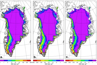
The fields and temporal variations of the annual ice sheet averaged amount of refrozen mass (Er) calculated by RACMO2 and MAR are presented in Figs. 1 and 2. They show that refreezing in RACMO2 and MAR agree reason-ably well although regionally differences occur. A detailed discussion of both fields with respect to the parameteriza-tions is given in Sect. 4. Figure 1 shows that most refreezing occurs along the margins, where most melt occurs (Fig. 3b). In the widest ablation area (western ice margin) the amount of refrozen mass is limited by the rapid removal of the win-ter accumulated snow pack above bare ice at the beginning of summer, making pore space the limiting factor for refreezing. Most refreezing occurs on the wet south and south-eastern margins, where pore volume is much larger. The amount of refreezing just below the equilibrium line is considerable, see e.g. the local maximum on the western ice margin, and is re-lated to multiple cycles of melt and refreezing.
Due to the lack of refreezing observations, the modelled refreezing cannot directly be robustly validated. An indica-tion of how well the models perform with respect to refreez-ing is given by validation of the snow characteristics for sin-gle locations with in situ observations, and for the spatial distribution, by validation of the surface mass balance field
and its components to satellite observations. For single loca-tions Crocus and SOMARS are compared to observaloca-tions by Greuell and Konzelman (1994); Lefebre et al. (2003); jmer and Hock (2008). Greuell and Konzelman (1994); Rei-jmer and Hock (2008) validate modeled snow temperatures and show that SOMARS is capable of modeling vertical pro-files and temporal variations in snow temperature (Figs. 8 and 9 of Greuell and Konzelman, 1994, Fig. 5 of Reijmer and Hock, 2008). Fig. 5 of Reijmer and Hock (2008) also shows that incorporating refreezing is necessary to obtain the cor-rect temporal variability in snow temperature. Lefebre et al. (2003) show that Crocus is capable of modeling water con-tent and snow density at the Swiss ETH camp in western Greenland (their Figs. 8 and 9). Ettema et al. (2009) show a good comparison of the RACMO2 SMB with in situ obser-vations (correlation coefficient R=0.95, their Fig. S2). They also show good correlation with observations for the compo-nents of precipitation (R=0.9) and melt, with modeled av-erage ablation along a transect on the western ice margin of 1417 mm w.e. yr−1versus observed 1413 mm w.e. yr−1. Fet-tweis et al. (2005, 2011) evaluate MAR SMB by compar-ing modeled and observed (derived from satellite brightness temperature data and in situ observations) melt extent and number of melt days. In Fettweis et al. (2011) RACMO2 is included in the comparison. Although some biases are present, which are partly ascribed to satellite data process-ing issues and partly to model specific issues, RACMO2 and MAR show good spatial and temporal agreement with the satellite observed melt extent. Spatial agreement varies be-tween R=0.88 and 0.95 depending on satellite retrieval al-goritm, and the number of melt days corresponds 97 % of the cases with in situ observations. Furthermore, Van den Broeke et al. (2009) and Rignot et al. (2011) show good agreement between the ice sheet averaged RACMO2 and GRACE (Gravity Recovery and Climate Experiment satel-lites) derived monthly mass balance variability (R=0.99, Fig. 1 in Van den Broeke et al., 2009). The capability of both models to reproduce the subsurface fields of tempera-ture, density and water content in combination with the good spatial correspondence of the SMB and melt extent with ob-servations provides confidence in the modeled refreezing.
3.3 Input data
We force the various parameterizations with the following input fields from RACMO2 and MAR: monthly snowfall, melt, rain, and, depending on the parameterization, surface temperature and net surface energy budget. Annual values of
Pr are then calculated and Eq. (2) applied to annual values ofWrto provide annual values ofEr. The parameterizations will be evaluated against RACMO2 fields unless stated oth-erwise. Note that the annual values are based on January to December monthly means or sums.
Fig. 1. Period (1958–2008) averaged anual sums of refrozen mass (Er) as modelled in (a) RACMO2, (b) MAR, and their difference (c) (MAR – RACMO2).
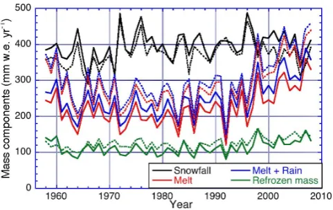
Fig. 2. Time series of ice sheet averaged annual sums of snowfall (C), melt (M), melt plus rain (Wr), and refrozen mass (Er) as mod-elled in RACMO2 (solid lines) and MAR (dashed lines).
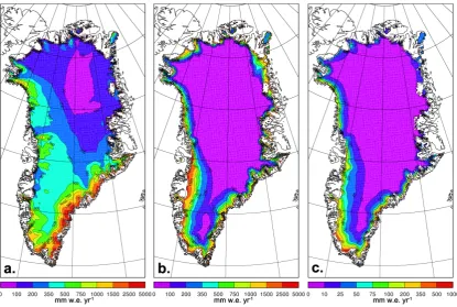
pronounced feature in Fig. 3a is the high snowfall over the southeast. The snowfall pattern is determined by the large scale circulation around Greenland and the ice sheet topog-raphy: the Icelandic Low advects moist oceanic air west-ward to the GrIS, where it rises steeply from sea level to 2.5 km height. Note that only a small part of the ice sheet receives on average more than 2 m w.e. per year and no point receives on average more than 5 m w.e. per year.
Snow-fall in MAR is on average smaller (366.9 mm w.e. yr−1 vs. 391.1 mm w.e. yr−1), with largest differences (>-70%) with RACMO2 on the southeast coast.
In RACMO2 about 50 % (70 %) of the total melt (runoff) occurs below the equilibrium line along the ice margin (Fig. 3b), and about 8 % (8 %) within about 10 km of the equilibrium line. The widest melt zone is located in the west. Total melt (runoff) in MAR is larger than in RACMO (234.8 (135.7) mm w.e. yr−1vs. 196.0 (108.3) mm w.e. yr−1), the spatial distribution is similar. Rainfall in both models is concentrated on the southern margins of the ice sheet (Fig. 3c). The percentage of the total precipitation falling as rain can be considerable (up to 50 %), and occasionally rain occurs at elevations over 2000 m, especially on the southern part of the ice sheet. Therefore, taking rain into account may (locally) have a significant impact on the estimated refreez-ing (see Sect. 4.2).
Fig. 3. Period (1958–2008) averaged anual sums of (a) snowfall (C) (b) melt (M), and (c) rain as modelled in RACMO2. Note the different scale in panel c.
The surface temperature shows the well-known decrease of temperature with height and elevation (Fig. 4). The
−15◦C isotherm corresponds to an altitude of about 1500 m (equilibrium line) on the western margin, and elsewhere ranges from sea level up to 2000 m. The annual average tem-perature on the GrIS is−24.3◦C (RACMO2), and varies be-tween−26.2◦C and−22.3◦C (Fig. 5). MAR is on average 0.4◦C warmer. Over the past 20 yr, surface temperature on the ice sheet has increased by about 2.5◦C; the first decade of the model period exhibits similarly high temperatures, al-though inter-annual variability was much larger than during the last decade.
4 Results
First a comparison will be made of the parameterizations as formulated in their original papers forced by and compared to both models, RACMO2 and MAR, in the absence of ob-servations. Then the input parameters will be varied and the effect on calculated amount of refreezing discussed. In these tests the parameterizations will be forced with and evaluated against RACMO2 fields.
4.1 Comparison
4.1.1 Time series
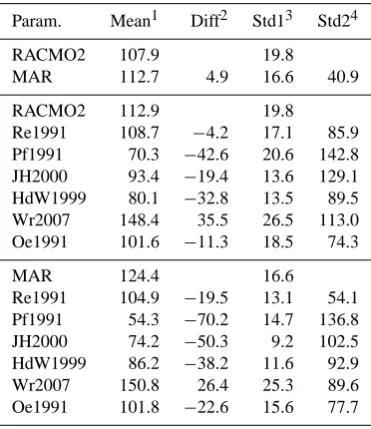
Figures 2 and 6 show that the inter-annual variability in modelled and parameterized values of Er are very similar for most methods. The absolute values, on the other hand, exhibit a large range around RACMO2 and MAR, with mean differences (Diff) ranging from −70.2 mm w.e. yr−1 (−56.4 %) to 35.5 mm w.e. yr−1 (+31.4 %) (Table 2). The average difference between RACMO2 and MAR is small (4.9 mm w.e. yr−1) and is only partly the result of differ-ences in snow model formulation. The atmospheric forcing in RACMO2 and MAR differs as well. Over the largest part of the ice sheet, i.e. the higher parts,Eris limited byWr. In these higher areas the correspondence between the models and the parameterizations is good (see next Section). In the models, because of this, a strong correlation exists between ice sheet annual averagedM(orM+ rain) andEr. The differ-ences in temporal variability and absolute amount in Fig. 6 are therefore mainly determined by the lower areas of the ice sheet, whereEris at least partly determined byPr.
Fig. 4. The period (1958–2008) average annual mean surface tem-perature (Ts) as modelled in RACMO2. The−15◦C isotherm cor-responds to an altitude of about 1500 m (equilibrium line) in the ablation area on the western margin, and elsewhere ranges from sea level up to 2000 m.
Fig. 5. Time series of ice sheet averaged annual averaged surface temperature (Ts, black) and temperature factor used in Eq. (7) (red) based on RACMO2 (solid lines) and MAR (dashed lines) fields. Note the reversed axis on the right hand side.
run off. Although JH2000 is the most physically based pa-rameterization, and in that sense best comparable to the models, the refreezing differs significantly from RACMO2 and even more from MAR. The absolute amount com-pared to RACMO2 (MAR) is lower by 17 % (40 %), as is the temporal variability (Std1), by 31 % (45 %). Of all pa-rameterizations the average difference with RACMO2 and
Fig. 6. Time series of ice sheet averaged annual sums of refrozen mass (Er) as modelled using the presented parameterizations. Using (a) RACMO2 and (b) MAR input fields.
MAR is smallest in Re1991 (Diff= −4.2 mm w.e. yr−1 and
−19.5 mm w.e. yr−1, respectively, Table 2). In Re1991, re-freezing is determined by either the annual average snowfall
C, or melt M (Eqs. 2 and 3). The value of Pmax=0.6 is obviously well chosen to represent the fraction ofC that is refrozen in the area wherePmax·C limits the amount of re-freezing.
Oe1991 also corresponds well with RACMO2 and MAR (Diff=11.3 mm w.e. yr−1 and 22.6 mm w.e. yr−1, respec-tively, Table 2). This is surprising since the formulation of
Table 2. Statistics of the different parameterizations compared to RACMO2 (second part) and MAR (third part). First part com-pares RACMO2 and MAR (MAR-RACMO2) for points where both models define ice. Mean1= ice sheet and period (1958–2008) aver-aged annualEr; Diff2= difference of Mean with an RCM; Std13= a measure for the temporal variability; Std24= a measure for the spatial variability in the difference. All values are expressed in mm w.e. yr−1.
Param. Mean1 Diff2 Std13 Std24
RACMO2 107.9 19.8
MAR 112.7 4.9 16.6 40.9
RACMO2 112.9 19.8
Re1991 108.7 −4.2 17.1 85.9 Pf1991 70.3 −42.6 20.6 142.8 JH2000 93.4 −19.4 13.6 129.1 HdW1999 80.1 −32.8 13.5 89.5 Wr2007 148.4 35.5 26.5 113.0 Oe1991 101.6 −11.3 18.5 74.3
MAR 124.4 16.6
Re1991 104.9 −19.5 13.1 54.1 Pf1991 54.3 −70.2 14.7 136.8 JH2000 74.2 −50.3 9.2 102.5 HdW1999 86.2 −38.2 11.6 92.9 Wr2007 150.8 26.4 25.3 89.6 Oe1991 101.8 −22.6 15.6 77.7
1Mean=1 nnyr1
P
i,jPyrEr(i, j, yr).i, jis the ice sheet grid
point at yearyrin period 1958–2008,nis the total number of grid points, andnyris the total number of years, for any
parameterization or RCM.
2Diff=Mean – Mean RCM
3Std1= r
1 nyrPyr
h 1
nPi,jEr(i, j, yr)−Meani2
4Std2= r 1 n P i,j h 1 nyr P
yrEr(i, j, yr)−nyr1 P
yrEr,RCM(i, j, yr)
−Diffi2
the case for the other parameterizations,Wr is the limiting factor over the remainder of the ice sheet, notPr.
The differences between the parameterizations when forced with RACMO2 or MAR are small (except for Pf1991 and JH2000) and can be explained by the on average higher amount ofM, higherTsand lower amount ofCin MAR. The larger differences in Pf1991 and JH2000 are due to the higher
Mand lowerC, both resulting in a smaller second term on the r.h.s. of Eqs. (4) and (5) and as a result lower amount of refreezing.
4.1.2 Areal distribution
The spatial fields ofErof RACMO2 and MAR show reason-able agreement (Std2= ∼40.9 mm w.e. yr−1, Table 2). The visible regional differences (Fig. 1c) can partly be explained by differences in snow model formulation and partly by the atmospheric forcing. Over most of the ice sheet MAR
ex-hibits more refreezing than RACMO2, which is due to the larger value for irreducible water content in MAR (6 % vs. 2 %). The different albedo formulations result in differences in timing and amount of melt. This is caused by the density of the snow surface (which determines the albedo in RACMO2) reacting slower to temperature changes than the surface snow grain characteristics (which determine the albedo in MAR). Enhanced by the melt-albedo feedback, melt occurs earlier and in slightly larger amounts in MAR. This signal is en-hanced by the sub freezing snow temperatures in spring, and by the larger delay between runoff and meltwater produc-tion in MAR compared to RACMO2. In MAR, the meltwater produced during the warmest hours of the day can refreeze during the following night, while in RACMO2 the meltwa-ter immediately runs off. In the areas where bare ice is ex-posed in the melt season, RACMO2 shows less refreezing than MAR due to a smaller minimum thickness of the upper-most snow layer in MAR (<1. cm vs.∼6.5 cm). As a result, snow disappears earlier and it takes longer to form a new layer of snow on ice in RACMO2. In addition, the bare ice albedo is lower in MAR (0.4-0.45 vs. 0.45-0.5) resulting in more melt production. In the areas where more refreezing occurs in RACMO2 compared to MAR, also more melt oc-curs, which in the north and southeast is the result of higher temperatures in RACMO2.
Comparing the spatial distributions based on the param-eterizations with the RCM refreezing shows significant dif-ferences (Fig. 7, Table 2). Note that Fig. 7 presents the spa-tial differences with respect to RACMO2. Spaspa-tial differences with respect to MAR are similar. In general, all parameteri-zations show small differences with the models in the higher parts of the ice sheet (<10 mm w.e.), whereWris the limiting factor for refreezing. For the parameterizations that take rain into account, the difference is zero (Fig. 7c, d, e), whereas the others show small negative differences in the order of the annual amount of rain. In the higher parts of the abla-tion zones refreezing in RACMO2 and MAR is reasonably high, which is the result of multiple cycles of melt/refreezing. These are not explicitly taken into account in the parameter-izations. The largest differences are once more found at the margins of the ice sheet, where most of the refreezing occurs. In these areasEr is mainly determined byPr, not Wr. The largest underestimation of refreezing compared to the models is found in Pf1991, which does not allow refreezing to occur below the runoff line, i.e. along the ice margins. Differences between MAR and RACMO2 forced parameterizations are explained by differences inWr for HdW1999, Wr2007 and Oe1991, while for the others the differences inCandM in determiningPralso play a role.
In RACMO2 and MAR,Pris not set by a given snow depth and determined more by the modelled snow temperature, re-sulting in lower values ofEr.
HdW1999 make use of a fixed depth of 2 m w.e. for the thermally active layer. On the south and southeast margin, this value is smaller than snowfallCresulting in lower values of Pr, limiting Er. Although Wr2007 also uses a constant value of the thermally active layer (5 m w.e.), this value is on average larger thanC and therefore does not explain the smaller values of Er on the southeast margin. The smaller difference between the models and Wr2007 in these areas is likely caused by a different representation of the cold content by using the integrated area between standard profiles of the winter and summer snow temperature instead of using the annual average temperature.
Based on Table 2, the best correspondence with RACMO2 (lowest Std2) is found for Oe1991, followed by Re1991 and HdW1999. For MAR the best correspondence is found for Re1991, followed by Oe1991 and HdW1999. Although the principles on which Pf1991 and especially JH2000 are based are the most similar to RACMO2 and MAR, the spa-tial correspondence is poorest (highest Std2 values, Table 2). Note that the spatial correspondence between RACMO2 and MAR is better, and the average difference between them smaller than compared to any of the parameteriza-tions (Diff=4.9 mm w.e. yr−1, Std2= ∼40.9 mm w.e. yr−1, Table 2). Only Re1991 forced with RACMO2 results in a smaller Diff. The good agreement between RACMO2 and MAR is especially interesting since the differences between them are only partly the result of differences in the snow model and partly due to differences in atmospheric forc-ing. In contrast, differences between parameterizations and RACMO2/MAR are solely due to the refreezing formulation.
4.2 Sensitivity experiments
We investigate the impact on the calculated amount of re-freezing of varying the different parameters in the parame-terizations: the period of averaging, the in- or exclusion of rain, as well as more model specific parameters such as the depth of the thermally active layer, temperature, yes or no capillary water, and density. The tests are described below and statistics are presented in Table 3. In these tests forcing field come from RACMO2 and the results will be compared to refreezing as calculated in RACMO2.
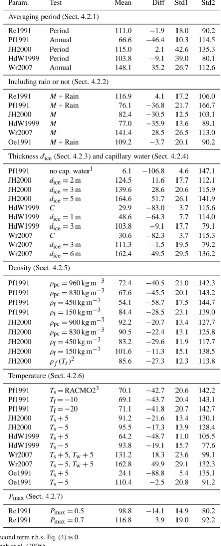
Table 3. Tests of the input variables of the parameterizations. RACMO2 input fields are used. Reference statistics are given in Ta-ble 2. Headings are as in TaTa-ble 2, Diff and Std2 are with respect to RACMO2 refreezing, test refers to change compared to reference, numbers between brackets denote sections where experiments are discussed.
Param. Test Mean Diff Std1 Std2
Averaging period (Sect. 4.2.1)
Re1991 Period 111.0 −1.9 18.0 90.2
Pf1991 Annual 66.6 −46.4 10.3 114.5
JH2000 Period 115.0 2.1 42.6 135.3
HdW1999 Period 103.8 −9.1 39.0 80.1
Wr2007 Annual 148.1 35.2 26.7 112.6
Including rain or not (Sect. 4.2.2)
Re1991 M+ Rain 116.9 4.1 17.2 106.0 Pf1991 M+ Rain 76.1 −36.8 21.7 166.7
JH2000 M 82.4 −30.5 12.5 103.1
HdW1999 M 77.0 −35.9 13.6 89.1
Wr2007 M 141.4 28.5 26.5 113.0
Oe1991 M+ Rain 109.2 −3.7 20.1 90.2 Thicknessdice(Sect. 4.2.3) and capillary water (Sect. 4.2.4)
Pf1991 no cap. water1 6.1 −106.8 4.6 147.1 JH2000 dice=2 m 124.5 11.6 17.7 112.1 JH2000 dice=3 m 139.6 28.6 20.6 115.9 JH2000 dice=5 m 164.6 51.7 26.1 141.9
HdW1999 C 29.9 −83.0 3.7 115.6
HdW1999 dice=1 m 48.6 −64.3 7.7 114.0 HdW1999 dice=3 m 103.8 −9.1 17.7 79.1
Wr2007 C 30.6 −82.3 3.7 115.3
Wr2007 dice=3 m 111.3 −1.5 19.5 79.2 Wr2007 dice=6 m 162.4 49.5 29.5 136.2 Density (Sect. 4.2.5)
Pf1991 ρpc=960 kg m−3 72.4 −40.5 21.0 142.3 Pf1991 ρpc=830 kg m−3 67.6 −45.5 20.1 143.2 Pf1991 ρf=450 kg m−3 54.1 −58.7 17.5 144.7 Pf1991 ρf=150 kg m−3 84.4 −28.5 23.1 139.0 JH2000 ρpc=900 kg m−3 92.2 −20.7 13.4 127.7 JH2000 ρpc=830 kg m−3 90.5 −22.4 13.1 125.8 JH2000 ρf=450 kg m−3 83.2 −29.6 11.9 117.7 JH2000 ρf=150 kg m−3 101.6 −11.3 15.1 138.5 JH2000 ρf(Ts)2 85.6 −27.3 12.3 113.8 Temperature (Sect. 4.2.6)
Pf1991 Ts=RACMO23 70.1 −42.7 20.6 142.2 Pf1991 Tf= −10 69.1 −43.7 20.4 143.1 Pf1991 Tf= −20 71.1 −41.8 20.7 142.7 JH2000 Ts+5 91.2 −21.6 13.4 130.1 JH2000 Ts−5 95.5 −17.3 13.9 128.4 HdW1999 Ts+5 64.2 −48.7 11.0 105.5 HdW1999 Ts−5 93.8 −19.1 15.7 77.6 Wr2007 Ts+5,Tw+5 131.2 18.3 23.6 99.1 Wr2007 Ts−5,Tw+5 162.8 49.9 29.1 132.3 Oe1991 Ts+5 24.1 −88.8 5.4 135.1 Oe1991 Ts−5 110.4 −2.5 20.8 91.2
Pmax(Sect. 4.2.7)
Re1991 Pmax=0.5 98.8 −14.1 14.9 80.2 Re1991 Pmax=0.7 116.8 3.9 19.0 92.2 1Second term r.h.s. Eq. (4) is 0.
2Reeh et al. (2005).
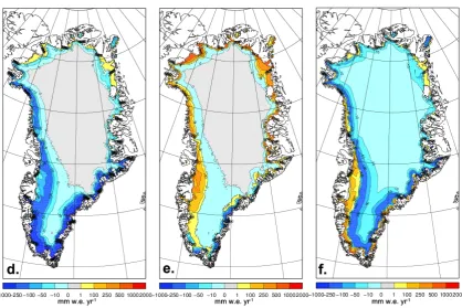
Fig. 8. Difference in refreezing when including rain inWr(Yes – No) for JH2000 (a) and HdW1999 (b), using RACMO2 input fields.
Fig. 10. Difference in refreezing when including capillary water inPr. Both panels show JH2000 minus HdW1999 (Yes – No). (a)dice=C, (b)dice= 2 m, using RACMO2 input fields.
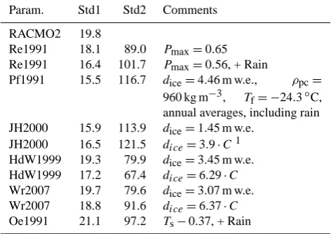
Table 4. Statistics of the different parameterizations compared to RACMO2 after tuning. Headings are as in Table 2, comments refers to changes in parameter setting compared to the refer-ence (Table 2). In all experiments Mean = 112.9 mm w.e. yr−1and Diff = 0.0 mm w.e. yr−1.
Param. Std1 Std2 Comments
RACMO2 19.8
Re1991 18.1 89.0 Pmax=0.65 Re1991 16.4 101.7 Pmax=0.56, + Rain
Pf1991 15.5 116.7 dice=4.46 m w.e., ρpc= 960 kg m−3, Tf= −24.3◦C, annual averages, including rain JH2000 15.9 113.9 dice=1.45 m w.e.
JH2000 16.5 121.5 dice=3.9·C1
HdW1999 19.3 79.9 dice=3.45 m w.e. HdW1999 17.2 67.4 dice=6.29·C
Wr2007 19.7 79.6 dice=3.07 m w.e. Wr2007 18.8 91.6 dice=6.37·C
Oe1991 21.1 97.2 Ts−0.37, + Rain
1only in first term r.h.s. Eq. (5).
4.2.1 Annual or period averages
The parameterizations presented in Sect. 2 are based on ei-ther annual average values ofC,Mand/orTs, or period mean (1958–2008) annual values (except Oe1991). The result is an annual Pr that is either constant throughout the calcu-lated period, or annually variable. The latter is the physically most correct approach and applied by Re1991, JH2000 and HdW1999. Pf1991 and Wr2007 make use of period average
Pr (Table 1). Pf1991 motivated his choice by limited avail-able information, while Wr2007 based their parameterization on typical profiles ofTsn at the end of winter and summer that were best represented by multi-year averages ofTs and Tw determined from snow/ice temperature profile measure-ments.
Fig. 11. Difference in refreezing when changing the density factor in JH2000 by changingρf=300 kg m−3(Eq. 5) to (a)ρf=150 kg m−3, (b)ρf=450 kg m−3, and (c)ρf(Ts) (Reeh et al., 2005) (test minus reference), using RACMO2 input fields. Note the reversed color scales in panels (b) and (c).
explained by the fact that withdice=5 m w.e., the refreezing over most part of the ice sheet is limited byWrand not byPr. Thus, as long as changes inPr do not result in a significant larger area wherePr exceedsWr,Erwill not change much when changingPr. In Re1991Pr is determined by C. Us-ing a period averageCresults in a larger dependency onM. Using period averages, HdW1999 and JH2000 are also more determined by variations inM. In these parameterizations the correspondence with RACMO2 increases due to the correla-tion betweenM andErin RACMO2. Note that HdW1999, which is a parameterization very similar to Wr2007, is more sensitive to changes inPr. This is caused by their choice of dice=2 m w.e. leading to an on average lowerPr. The im-pact of varyingdice will be discussed in more detail below. Using period averages, HdW1999 and JH2000 are more de-termined by variations inM. As a result, both show an in-crease inEr, corresponding to the increase in M, which is larger than found in RACMO2.
4.2.2 Refreezing of rain
The amount of refreezing (Er) is (partly) determined by the available amount of water including rain (Wr). However, not all parameterizations take rain falling on cold snow into ac-count in their estimate ofWr. Pf1991, Re1991 and Oe1991 assume the contribution of rain to be negligible, because rain
constitutes only a small fraction of the total amount of pre-cipitation. In RACMO2, about 6 % of the annual amount of precipitation over the ice sheet falls as rain, with the largest percentages (up to 50 %) on the southern ice margins. There-fore, refreezing of rain may locally constitute a significant contribution to the total.
Fig. 12. Difference in refreezing when using different temper-ature descriptions (Wr2007 – HdW1999 with dice=3 m), using RACMO2 input fields.
the areas where available liquid water is the limiting factor, which is just above the equilibrium line.
4.2.3 Depth of the thermally active layer
All the parameterizations tested in this study, except Oe1991, use an estimate of the depth of the thermally active layer (dice). Oe1991 implicitly assumedice= 2 m snow by using the average snow temperature of a 2 m thick layer. The impact of varyingTswill be discussed in more detail below. Parameter-izations Pf1991, JH2000 and Re1991 assume thatdiceequals annual snowfallC, whereas HdW1999 and Wr2007 assume a constant value fordiceof 2 m w.e. and 5 m w.e., respectively. In the tests we varydice, or usedice=C. Unfortunately, the maximim depth at which refreezing occurs in RACMO2 is not stored and can therefore not be used as a reference or inputdicefield.
The amount of refreezing changes significantly when changingdice as can be seen in Table 3 and Fig. 9. Figure 9 shows the difference inEr when using different values of dice, and illustrates that whendice increases, refreezing in-creases, the latter becoming more and more limited by the available amount of liquid waterWr. Using a constantdice, JH2000, HdW1999 and Wr2007, can be tuned to best repre-sent the ice sheet and period averaged RACMO2 refreezing (Table 4). Wr2007 and HdW1999 show the smallest mean difference and the best correspondence in temporal and spa-tial variability to RACMO2 whendiceis about 3 m w.e. (3.07
and 3.45 m w.e., respectively), while JH2000 shows the best correspondence whendice=1.45 m w.e.
In all experiments, usingdice=C drastically reduces the amount of refreezing (Fig. 9b). The reason is that period aver-agedCis only 0.39 m w.e. yr−1in RACMO2. Usingdice=C results in smallerProver those parts of the ice sheet where annual average C is smaller than 3 m w.e. (Fig. 3a), which is virtually everywhere. In addition, the inter-annual vari-ability almost vanishes, and the spatial correspondence with RACMO2 decreases. JH2000 is the least affected by this choice because they include refreezing of capillary water, which does not depend on the depth of the thermally ac-tive layer. Multiplying C with a constant factor increases the amount of refreezing and the temporal variability. Table 4 presents the factors giving best correspondence to RACMO2 for JH2000, HdW1999 and Wr2007. The results are similar to tuning a constantdice.
4.2.4 Capillary water
Pf1991 and JH2000 are the only parameterizations that specifically take into account the refreezing of capillary wa-ter at the end of the melt season (second wa-term r.h.s. Eqs. 4 and 5). We tested the impact by removing this term in Eqs. (4) and (5). Note that removing the capillary water in JH2000 equals using HdW1999 with the same dice as JH2000. In-cluding capillary water increases the amount of refreezing (Table 3). It also results in a larger temporal variability. How-ever, although RACMO2 also includes the contribution of capillary water, including it in the parameterizations does not result in a better spatial agreement with RACMO2.
Figure 10 shows that capillary water is a significant con-tributor to refreezing in areas were melt M does not ex-ceed the amount of snowfallC. This is especially the case in Pf1991 where, due to the mask formulation and the use of Tf= −15◦C, the remaining cold content is very small, resulting in only a small area where refreezing occurs. In JH2000, the areas where the difference is zero are those whereM exceeds C and those where Pr minus the possi-ble capillary contribution is larger than M. In case dice is constant, the latter area is larger becausePrremains larger compared to the case wheredice=C, since over large areas of the ice sheetC is on average smaller than 2 m w.e. (see Fig. 3a).
4.2.5 Density
When including the capillary water content, the additional amount of refreezing that may occur depends on the cho-sen densities. JH2000 (Eq. 5) use a pore close-off density
Fig. 13. Fraction of refreezing over snowfall (Er/C) from RACMO2 (a) and MAR (b) fields.
actual pore close of density, and 960 kg m−3. Tests with the density factor are presented in Table 3 and Fig. 11.
Increasing the density factor, either by increasing ρpc or decreasing ρf, results in a larger amount of refreez-ing. The increase is largest in areas around the equilibrium line. Increasing the density factor further results in a larger inter-annual variability and less spatial correspondence with RACMO2 in case of JH2000 and more in case of Pf1991 (Ta-ble 3). Changingρfhas the largest impact, but the change has to be considerable to have a significant effect. This is because changing density only has effect in areas were less than the annual amount of snowfallCmelts away, and wherePris the limiting factor, notWr.
Reeh et al. (2005) present ρf as a function of Ts based on observations on the GrIS. Using this function in JH2000, the effect is similar to using a higher constant value ofρf, i.e. a reduction in amount of refreezing and an increase in spatial correspondence to RACMO2 (Fig. 11c, Table 3). Us-ing RACMO2 output,ρfas a function of altitude, snowfall or temperature can be derived. However, the skill of the re-sulting functions is limited, the scatter large and largest in lower elevation areas with higher temperatures and higher snow fall amounts. These are the areas where the differences between RACMO2 refreezing and the parameterizations is largest (Fig. 7). This explains why including such functions does not improve the correspondence between RACMO2 and JH2000.
4.2.6 Temperature
In several parameterizations temperature is used as a mea-sure for the cold content of the snow. Except for Pf1991, all parameterizations were forced by RACMO2 surface temper-aturesTs. Pf1991 uses a representative value of the firn tem-perature at the firn limit (−15◦C). The impact of the param-eterized refreezing to variations the temperature indicates in fact how well this temperature represents the cold content of the snow.
Table 3 shows that Pf1991 and JH2000 are not very sen-sitive to reasonable changes inTswhile HdW1991, Wr2007 and Oe1991 are more sensitive. In Oe1991 changes inErdue
4.2.7 Pmax
Compared to RACMO2, Pr=0.6C represents the amount and temporal variability in refreezing well in areas where
Pris the limiting factor (Table 2). Tuning results in an even better correspondence in average amount, although the re-sulting value ofPmaxdoes not deviate much from 0.6 (0.65, Table 4). When including Rain, a slightly lower value results in the best correspondence (Pmax= 0.56). In both cases (with
or without rain), increasingPmaxincreases the amount of re-freezing below the elevation whereWr is the limiting fac-tor and increases the area whereWris the limiting factor. It also increases the temporal variability and decreases the spa-tial correspondence with RACMO2. DecreasingPmaxresults in the opposite: it decreases the temporal variability and in-creases the correspondence with RACMO2.
From RACMO2 (and MAR) fields ofC andEr, the frac-tion ofC that is refrozen can be calculated (Fig. 13). Inter-esting feature in this figure is the northern marginal areas where the fraction is larger than 1 and thus more than the annual amount of snowfall refreezes. This is the result of multiple cycles of melt and refreezing of the same snow/ice. This happens over the whole GrIS, but in areas where little or no runoff takes place, andC is small, this can result in
Er/C >1. Since the cold snow pack warms up due the en-ergy provided by refreezing, the increase in melt over the pe-riod 1958–2008 (Fig. 2) will degrade the refreezing capacity in these areas to the point that runoff starts. In contrast, in the southeastern marginal zoneEris small compared toC. Only on the western margin of the ice sheet are there significant areas where the fraction is about 0.6, similar to the value of
Pmaxmeasured by Braithwaite et al. (1994) in this area. The ice sheet average value of Er/C is 0.28 (MAR 0.34); this high value is the result of the multiple cycles of melt and re-freezing. The higher value in MAR is due to the on average larger amount of Er and lower amount ofC. Whether the modeledEr/C is reasonable is difficult to determine given
the lack of observations for validation.
5 Summary and conclusions
In this study we applied several parameterizations that cal-culate the annual amount of refreezing to the Greenland ice sheet. In the absence of refreezing observations we compare the results to output of the RACMO2 and MAR regional cli-mate models, that both include an explicit scheme to calcu-late retention and refreezing as a function of snow depth, temperature and density. The parameterizations are forced with output from the same models for consistency. Almost all refreezing parameterizations discussed here use tempera-ture and an estimate of the depth of the thermally active layer to determine the cold content of the snow. In RACMO2 and MAR, water may percolate to any depth depending on the vertical temperature and density distribution in the snow/firn.
Note that none of the parameterizations, or the regional cli-mate models, explicitly include heterogeneous infiltration (piping) of water, a process known to be important for heat-ing cold firn (Marsh and Woo, 1984; Pfeffer and Humphrey, 1996).
In the absence of observations we use RACMO2 as ref-erence. Refreezing in RACMO2 and MAR agree well; an-nual, period average (1958–2008) and ice sheet averaged values differ by ∼4.5 %, temporal variability is similar (Std1 = 19.8 mm w.e yr−1 and 16.6 mm w.e yr−1, respec-tively) and spatial correspondence reasonably good (Std2=
40.9 mm w.e. yr−1, Table 2). Differences are explained by the chosen amount of irreducible water content (6 % MAR and 2 % RACMO2), the albedo formulation, the minimum thick-ness of the uppermost snow layer (<1 cm MAR and∼6.5 cm RACMO2), and differences in atmospheric temperature and precipitation. All in all, correspondence between both mod-els is better than with any of the parameterizations. This provides confidence in the RCMs since differences between MAR and RACMO2 are only partly the result of the snow model formulation and partly due to the atmospheric forc-ing (mainly temperature and precipitation). In contrast, dif-ferences between the parameterizations and RACMO2/MAR are solely due to the refreezing formulation.
The annual, period average (1958–2008) and ice sheet av-eraged amount of refreezing calculated with the different pa-rameterizations differs up to a factor 2 with RACMO2 and MAR (Table 2). The spatial fields show large differences as well, especially in the lower areas of the ice sheet (up to a factor 5). Janssens and Huybrechts (2000) also noted large differences in parameterized refreezing in these areas, which they related to the chosen depth of the thermally active layer. Our results confirm this large sensitivity as well as the large impact this has on refreezing in the marginal areas. Depend-ing on parameterization, usDepend-ing period or annual average in-put fields, changing inin-put temperature or density has a large impact on the results as well. All parameterizations can be tuned within realistic limits, to produce ice sheet and annual average amount of refreezing similar to RACMO2, but this does not necessarily result in better spatial correspondence (Table 4). After tuning, the temporal variability of Wr2007 and the spatial variability of HdW1999 are most similar to RACMO2.
amount of refreezing in Oe1991 depends on available energy and an average temperature over a 2 m snow layer. Oe1991 is very sensitive to changes in this temperature. However, Oe1991 was designed for application in an energy balance model that includes a simple snow model, in which the snow temperature changes when refreezing occurs. To obtain rea-sonable results in our test, the refreezing is limited to the total annual precipitationPtot. It is questionable whether Oe1991 will work similarly well in other settings and without those constraints.
The presented parameterizations and both models (RACMO2 and MAR) are based on the same principles and are on average in reasonable agreement. RACMO2 and MAR surface mass balance fields show good agreement with surface and satellite observations (Ettema et al., 2009; Van den Broeke et al., 2009; Fettweis et al., 2011). Furthermore, Greuell and Konzelman (1994); Lefebre et al. (2003); Reijmer and Hock (2008) show for single locations that SOMARS and Crocus are capable of realistically modeling the observed snow temperature, density and water content. In combination with the spatial correspondence between RACMO2 and MAR, this implicitly gives confidence in modeled refreezing. The lack of spatial correspondence between the different parameterizations and the models indicates that, at least in the parameterizations but likely in the models as well, not all processes are included or described adequately. For example, omitting piping may be important in the snow models in RACMO2 and MAR because it affects the depth at which refreezing occurs, thus affecting the vertical temperature and density distribution (Humphrey et al., 2012). It also indicates that it is unlikely that tuning the parameterizations to e.g. an observation results in a correct spatial distribution, or that the results are transferable to other locations and/or periods. A next step in the study of refreezing would be validation of available comprehensive snow models against observations; including the process of piping in these models; and using them in models such as RACMO2 and MAR to study the impact of refreezing on the GrIS surface mass balance.
Acknowledgements. We thank R. Fausto, T. Pfeffer, I. Janssens
and an anonymous referee for their constructive comments. This work is funded by the Utrecht University and the Netherlands Polar Programme. The ECMWF and KNMI are thanked for providing computing and data archiving support.
Edited by: J. L. Bamber
References
Bøggild, C.: Simulation and parameterization of superimposed ice formation, Hydrol. Process., 21, 1561–1566, 2007.
Bougamont, M., Bamber, J. L., and Greuell, W.: A surface mass balance model for the Greenland ice sheet, J. Geophys. Res., 110, doi:10.1029/2005JF000348, 2005.
Box, J., Bromwich, D., Veenhuis, B., Bai, L.-S., Stroeve, J., Rogers, J., Steffen, K., Haran, T., and Wang, S.-H.: Greenland Ice Sheet Surface Mass Balance Variability (1988-2004) from Calibrated Polar MM5 Output, J. Climate, 19, 2783–2800, 2006.
Braithwaite, R., Laternser, M., and Pfeffer, W.: Variations of near-surface firn density in the lower accumulation area of the Green-land ice sheet, Pakitsoq, West GreenGreen-land, J. Glaciol., 40, 477– 485, 1994.
Brun, E., Martin, E., V. Simon, C. G., and Coleou, C.: An energy and mass model of snow cover suitable for operational avalanche forecasting, J. Glaciol., 35, 333–342, 1989.
Brun, E., David, P., Sudul, M., and Brunot, G.: A numerical model to simulate snow-cover stratigraphy for operational avalanche forecasting, J. Glaciol., 38, 13–22, 1992.
Col´eou, C. and Lesaffre, B.: Irreducible water saturation in snow: Experimental results in a cold laboratory, Ann. Glaciol., 26, 64– 68, 1998.
Ettema, J., van den Broeke, M., van Meijgaard, E., van de Berg, W., Bamber, J., Box, J., and Bales, R.: Higher surface mass balance of the Greenland ice sheet revealed by high-resolution climate modeling, Geophys. Res. Lett., 36, doi:10.1029/2009GL038110, 2009.
Ettema, J., van den Broeke, M., van Meijgaard, E., and van de Berg, W.: Climate of the Greenland ice sheet using a high-resolution climate model – Part 2: Near-surface climate and energy balance, The Cryosphere, 4, 529–544, 2010a.
Ettema, J., van den Broeke, M., van Meijgaard, E., van de Berg, W., Box, J., and Steffen, K.: Climate of the Greenland ice sheet using a high-resolution climate model – Part 1: Evaluation, The Cryosphere, 4, 511–527, 2010b.
Fausto, R., Ahlstrøm, A., van As, D., Johnsen, S., Langen, P., and Steffen, K.: Improving surface boundary conditions with focus on coupling snow densification and meltwater retention in large-scale ice-sheet models of Greenland, J. Glaciol., 55, 869–878, 2009.
Fettweis, X.: Reconstruction of the 1979-2006 Greenland ice sheet surface mass balance using the regional climate model MAR, The Cryosphere, 1, 21–40, 2007,
http://www.the-cryosphere-discuss.net/1/21/2007/.
Fettweis, X., Gall´ee, H., Lefebre, F., and van Ypersele, J.: Green-land surface mass balance simulated by a regional climate model and comparison with satellite-derived data in 1990-1991, Cli-mate Dynamics, 24, 623–640, doi:10.1007/s00382-005-0010-y, 2005.
Fettweis, X., Tedesco, M., van den Broeke, M., and Ettema, J.: Melting trends over the Greenland ice sheet (1958-2009) from spaceborne microwave data and regional climate models, The Cryosphere, 5, 359–375, 2011,
http://www.the-cryosphere-discuss.net/5/359/2011/.
Gall´ee, H. and Schayes, G.: Development of a Three-Dimensional Meso-γprimitive equation model: katabatic winds simulation in the area of Terra Nova Bay, Antarctica, Mon. Weather Rev., 122, 671–685, 1994.
Gall´ee, H., Guyomarch, G., and Brun, E.: Impact of Snow Drift on the Antarctic Ice Sheet Surface Mass Balance: Possible Sensitiv-ity to Snow-Surface Properties, Boundary-Layer Meteorol., 99, 1–19, 2001.
Greuell, W. and Konzelman, T.: Numerical modelling of the en-ergy balance and the englacial temperature of the Greenland ice sheet. Calculations for the ETH-Camp location (West Green-land, 1155 m a.s.l.), Global and Planetary Change, 9, 91–114, doi:10.1016/0921-8181(94)90010-8, 1994.
Hanna, E., Huybrechts, P., Steffen, K., Cappelen, J., Huff, R., Shu-man, C., Irvine-Fynn, T., Wise, S., and Griffiths, M.: Increased Runoff from Melt from the Greenland Ice Sheet: A Response to Global Warming, J. Climate, 21, 331–341, 2008.
Herron, M. and Langway, C.: Firn densification: An empirical model, J. Glaciol., 25, 373–385, 1980.
Humphrey, N., Harper, J., and Pfeffer, W.: Thermal tracking of melt-water retention in Greenland’s accumulation area, J. Geophys. Res., 117, doi: 10.1029/2011JF002083, 2012.
Huybrechts, P. and de Wolde, J.: The Dynamic Response of the Greenland and Antarctic ice sheets to Multiple-century climate warming, J. Climate, 12, 2169–2188, 1999.
Janssens, I. and Huybrechts, P.: The treatment of meltwater re-tention in mass-balance parameterizations of the Greenland ice sheet, Ann. Glaciol., 31, 133–140, 2000.
Lefebre, F., Gall´ee, H., van Ypersele, J. P., and Greuell, W.: Modeling of snow and ice melt at ETH-Camp (West Green-land): A study of surface albedo, J. Geophys. Res., 108, 4231, doi:10.1029/2001JD001160, 2003.
Lefebre, F., Fettweis, X., Gall´ee, H., van Ypersele, J., Marbaix, P., Greuell, W., and Calanca, P.: Evaluation of a high-resolution re-gional climate simulation over Greenland, Climate Dynamics, 25, 99–116, 2005.
Lenaerts, J., van den Broeke, M., D´ery, S., van Meijgaard, E., van de Berg, W., Palm, S., and Rodrigo, J. S.: Modeling drifting snow in Antarctica with a regional climate model, part I: Methods and model evaluation, J. Geophys. Res., 117, doi:10.1029/2011JD016145, 2012.
Marsh, P. and Woo, M.: Wetting front and refreezing of meltwa-ter within a snow cover. 1. Observation in the Canadian Arctic, Water Resour. Res., 20, 1853–1864, 1984.
Oerlemans, J.: The mass balance of the Greenland ice sheet: sensi-tivity to climate change as revealed by energy balance modelling, The Holocene, 1, 40–49, 1991.
Paterson, W.: The Physics of Glaciers, Pergamon, 480 pp, 1994. Pfeffer, W. and Humphrey, N.: Determination of timing and location
of water movement and ice-layer formation by temperature mea-surements in sub-freezing snow, J. Glaciol., 42, 292–304, 1996.
Pfeffer, W., Illangasekare, T., and Meier, M.: Analysis and mod-elling of melt-water refreezing in dry snow, J. Glaciol., 36, 238– 246, 1990.
Pfeffer, W., Meier, M., and Illangasekare, T.: Retention of Green-land runoff by refreezing: implications for projected future sea level change, J. Geophys. Res., 96, 22117–22124, 1991. Reeh, N.: Parameterization of melt rate and surface temperature on
the greenland ice sheet, Polarforschung, 59, 113–128, 1991. Reeh, N., Fisher, D., Koerner, R., and Clausen, H.: An empirical
firn-densification model comprising ice lenses, Ann. Glaciol., 42, 101–106, 2005.
Reijmer, C. and Hock, R.: Internal accumulation on Storglaci¨aren, Sweden, in a multi-layer snow model coupled to a distributed energy- and mass-balance model, J. Glaciol., 54, 61–72, 2008. Rignot, E., Velicogna, I., van den Broeke, M., Monaghan, A., and
Lenaerts, J.: Acceleration of the contribution of the Greenland and Antarctic ice sheets to sea level rise, Geophys. Res. Lett., 38, doi:10.1029/2011GL046583, 2011.
Schneider, T. and Jansson, P.: Internal accumulation in firn and its significance for the mass balance of Storglaci¨aren, Sweden, J. Glaciol., 50, 25–34, 2004.
Trabant, D. and Mayo, L.: Estimation and effects of internal accu-mulation on five glaciers in Alaska, Ann. Glaciol., 6, 113–117, 1985.
Van de Berg, W., van den Broeke, M., Reijmer, C., and van Mei-jgaard, E.: Reassessment of the Antarctic surface mass balance using calibrated output of a regional atmospheric climate model, J. Geophys. Res., 111, doi:10.1029/2005JD006495, 2006. Van den Broeke, M., Bamber, J., Ettema, J., Rignot, E., Schrama, E.,
van de Berg, W., van Meijgaard, E., Velicogna, I., and Wouters, B.: Partitioning recent Greenland mass loss, Science, 326, 984– 986, 2009.
Van Dusen, M.: International Critical Tables of Numerical Data: Physics, Chemistry and Technology, chap. Thermal conductivity of non-metallic solids, 216–217, McGraw Hill, 1929.
Van Meijgaard, E., van Ulft, L., van de Berg, W., Bosveld, F., van den Hurk, B., Lenderink, G., and Siebesma, A.: The KNMI regional atmospheric climate model, version 2.1, KNMI Tech. Rep. 302, Royal Dutch Meteorological Institute (KNMI), De Bilts, the Netherlands, 2008.
Wright, A., Wadham, J., Siegert, M., Luckman, A., Kohler, J., and Nuttall, A.: Modeling the refreezing of meltwater as superimosed ice on a high Arctic glacier: A comparison of approaches, J. Geo-phys. Res., 112, 2007.
Yen, Y.-C.: Review of thermal properties of snow, ice and sea ice, Rep. 81-10, CRREL, Cold Reg. Res. and Eng. Lab., Hanover, N.H., 1981.