Open Access
Research
Pattern statistics on Markov chains and sensitivity to parameter
estimation
Grégory Nuel*
Address: Laboratoire Statistique et Génome, University of Evry, CNRS (8071), INRA(1152), 523, place des terrasses de I'Agora, 91034 Evry CEDEX, France
Email: Grégory Nuel* - [email protected] * Corresponding author
Abstract
Background: In order to compute pattern statistics in computational biology a Markov model is commonly used to take into account the sequence composition. Usually its parameter must be estimated. The aim of this paper is to determine how sensitive these statistics are to parameter estimation, and what are the consequences of this variability on pattern studies (finding the most over-represented words in a genome, the most significant common words to a set of sequences,...).
Results: In the particular case where pattern statistics (overlap counting only) computed through binomial approximations we use the delta-method to give an explicit expression of σ, the standard deviation of a pattern statistic. This result is validated using simulations and a simple pattern study is also considered.
Conclusion: We establish that the use of high order Markov model could easily lead to major mistakes due to the high sensitivity of pattern statistics to parameter estimation.
Background
In order to study pattern occurrences in biological sequences, simple frequencies are not relevant in most cases because of pattern overlapping structure as well as composition bias in the sequences. A common worka-round consists to compute the significance of an observa-tion assuming the sequence X = X1 ... Xᐍover the finite
alphabet . (size k) is generated according to an order m
≥ 1 homogeneous, stationary and ergodic Markov model. Let π (size km+1) defined by
π(w, a) = (Xm+1 = a|X1...Xm = w) ∀(w, a) ∈ m × (1)
be the parameter of this Markov model, Π its transition matrix (note that we have Π = π only if m = 1) and μ its stationary distribution (defined by μ × Π = μ).
We then introduce the pattern statistic defined by
where N is the random number of overlapping occur-rences (i. e. X = aababaaba contains three overlapping occurrences of aba but only two non-overlapping ones) of a given fixed pattern on the random sequence X and Nobs is an observation.
Published: 17 October 2006
Algorithms for Molecular Biology 2006, 1:17 doi:10.1186/1748-7188-1-17
Received: 07 April 2006 Accepted: 17 October 2006
This article is available from: http://www.almob.org/content/1/1/17 © 2006 Nuel; licensee BioMed Central Ltd.
This is an Open Access article distributed under the terms of the Creative Commons Attribution License (http://creativecommons.org/licenses/by/2.0), which permits unrestricted use, distribution, and reproduction in any medium, provided the original work is properly cited.
S N N N N
N N N N
= − ≥ ≥
≤ <
⎧ log ( ) [ ]
log ( ) [ ]
10
10
P E
P E
obs obs
obs obs
if if ⎨⎨
When π is known (and hence μ), several statistical meth-ods are available to compute S: exact computations [1-4], Gaussian [5,6], binomial [7,8], compound Poisson [9-11] or large deviations approximations [12]. But in general, the parameter π is not available and must be estimated. Let us denote by N0 (resp. N1) the (overlap) frequencies of all words of size m (resp. m + 1) in the sequence Y = Y1 ...
Yn, then the Maximum-Likelihood Estimator (MLE) of π is given by
and the MLE of μ (as a function of π) is therefore defined by × = where is the transition matrix
associ-ated to
We introduce now the following estimators
which are known to be asymptotically equivalent with the MLE when n is large.
The quality of parameter estimation depends both on the number of parameters to estimate (km+1 for an order m
Markov model) and of the length (n) of the homogeneous sequence used for their estimation. When the same sequence (or set of sequences) is used both for observed frequencies and parameter estimation, m should not be greater than h – 2 for a pattern of length h (as else, the observed frequency of the pattern will be included in the model). As literature often suggests to use the highest pos-sible order, it is hence common to consider m = 6 or more (for a DNA pattern of size h ≥ 8). Moreover, because of the homogeneity assumption of the model, the considered genomes have often to be segmented first. As a result, the sequences length used for parameter estimations are often dramatically reduced by such segmentation (e. g. n = 105
to n = 106 at the very best for DNA sequences). It is hence
quite common to encounter high order Markov models estimated on rather short sequences which could result in high sensitivity to parameter estimation.
Considering that Y is generated through a Markov model of parameter π, the main goal of this paper is to study the distribution of SN, the statistic S computed using the esti-mators μN and πN, and the consequences of its variability in projects using pattern statistics. We first present in details how the delta-method can be used to get a Gaus-sian approximation for the distribution of SN (using a binomial approximation to compute the pattern statis-tics). Then these approximations are validated through simulations and, at last, we consider a classical pattern
study (finding the most over-represented patterns of a given size) and we evaluate the detrimental effect of parameter estimations both in terms of true positive rate and rank accordance.
Materials and methods
Distribution of N = (N0, N1)
As the estimators defined in (4) are expressed as functions of N0 and N1 we first study their distribution. Using a Gaussian approximation, we have
where, for i, j ∈ {0, 1}, Ei ∈ , and Ci,j ∈ × with di = km+i. One can note that C
0,0 and C1,1 are
symmet-ric, and t (C
1,0) = C0,1 (where t is the matrix transpose
oper-ator).
In the stationary case, exact expression of E and C can be computed according to [5].
Expectation is simply given ∀w ∈ m by
E0(w) = (n - m + 1) μ(w) E1 (wa) = (n - m) μ(w)Π(w, a)
∀(w, a) ∈ m × (6)
In order to give more fluidity to this paper, the expression of the covariance matrix C have been moved in appendix A. Let us remark, before going forward that substituting N by E in (4) immediately gives
Delta method
Let us start with a simple case. We consider a single pattern which is over-represented (seen more than expected) so we have
where the function F+ also depends on the sequence
length ᐍ and the considered pattern.
If F+ is differentiate, the delta-method (a simple first order
Taylor expansion around N = E, see [13]) provides the fol-lowing approximation:
ˆ( , ) ( )
( ) ( , ) ( )
π w a wa
wb w a
b
m
= ∀ ∈ ×
∈
∑
N N1
1
3
ˆ
μ Πˆ μˆ Πˆ ˆ
π
μN N πN N
N
( ) ( ) ( , ) ( )
( ) ( , ) ( )
w w
n m w a
wa
w w a
m
=
− +0 1 = 10 ∀ ∈ ×
4
and
N
N
E E
C C C C
N E
0
1
0
1
0 0 0 1
1 0 1 1
⎡ ⎣ ⎢ ⎤
⎦ ⎥ ⎛
⎝ ⎜ ⎜ ⎜ ⎜
⎞
⎠ ⎟ ⎟ ⎟ ⎟
⎡ ⎣ ⎢ ⎤
⎦ ⎥ ⎡
⎣
N
N
, , ,
, ,
⎢⎢ ⎤
⎦ ⎥ ⎛
⎝ ⎜ ⎜ ⎜ ⎜
⎞
⎠ ⎟ ⎟ ⎟ ⎟
C
( )5
\di \di \dj
μE =μ πE = − π
− + ⎛
⎝⎜
⎞
⎠⎟
( )
and 1 1
1 7
n m
SN= − F N F N N N N≥N ( )
+ +
and hence, using (7) we have
for n large enough. The distribution of is therefore approximated by
(SN) ⯝ (S, σ2) (11)
with
In consequence, computing σ requires both to compute C (done in appendix A) and ∇F+ (E).
Single pattern
The exact expression of F+ is computable through many
different methods [1-4] but is too much complicated to derive explicitly ∇F+. To overcome this problem, we
pro-pose to consider an approximation of F+. As said in
intro-duction, many kind of approximations are available (Gaussian, binomial, compound Poisson or large devia-tions). In this paper, we have chosen to use a binomial approximation as it provides an expression which is ana-lytically differentiable and is known to be a good heuristic to the problem [8].
For a single non-degenerate pattern (i.e. a simple word) W = w1 ... wh (wi ∈ ) with h ≥ m - 1 we first denote by
P(N) = μN (w1 ... wm) × πN (w1 ... wm, wm+1) × ... × πN (wh-m ... wh-1, wh) (13)
the probability for W to occur at a given position in the sequence and then we get
where denotes the binomial distribution, with ᐍh = ᐍ
-h + 1 and w-here t-he β functions (complete and incom-plete) and their relation to the binomial cumulative distri-bution function are described in appendix B.
Note that if we consider non-overlapping occurrences instead of overlapping ones, we can still use a binomial
approximation for the distribution of N, but the expres-sion of P(N) is more complicated as it involves the auto-correlation polynome of the pattern [14]. This point is not developed in this paper.
Replacing μN and πN by their expression easily gives
where A1(wa) counts occurrences of the word wa in W = w1 ... wh and A0 (w) counts occurrences of the word w in w2 ... wh-1. Note that in the particular case where h = m - 1, all A0 (w) are null and we simply get (n - m + l) × P (N) = N1 (W).
Using the derivative properties of the incomplete beta function (see appendix B for more details) we hence get
so all we need is to compute ∇P(N).
For all (w, a) ∈ m × we have
and
If we denote by
P = μ (w1 ... wm) × π (w1 ... wm, wm+1) × ... × π (wh-m ... wh-1, wh) (19)
the true probability for W to occur at a given position in the sequence X then we get, using (7) in (13), that
for n large enough. We hence get
where tG = [tG
0 tG1] is defined by
S F F
F
t
N E
N E E E
− + − − ∇ +
( )
+
log ( ) ( ) ( )
ln( ) ( ) 10
10 9
S S F
F
t
N
N E E E
− − ∇ +
( )
+
( ) ( )
ln( )10 ( ) 10
ˆ
S
L
σ = ∇ + × × ∇+ +
( )
t F F
F
( ) ( )
ln( ) ( ) E C E
E 10
12
F P N P N N
N N h h h + ≥ = − + − ( ) ( ( , ( )) ) ( ( ), , ) ( ,
N A N N A
A
P obs obs
obs
β
β obs
1
o obs+1
14 ) ( ) P n m wa w A wa a A w w m ( ) ( ) ( ) ( ) ( ) ( ) N N N = − + ∈
∏
∏
∈ 1 1 15 1 0 1 0 ∇ − − + × ∇(
+ − −F P P
N N P
N N
h
h
( ) ( ) ( ( ))
( , ) ( )
N N N N
A A obs obs obs obs 11 1 16 β
))
∂ ∂ = − ×( )
P w A w w P ( ) ( ) ( ) ( ) ( ) NN0 N0 N
0 17 ∂ ∂ = − ×
( )
P w A wa wa P ( ) ( ) ( ) ( ) ( ) NN1 N1 N
1 18
P p
n m p
h m ( )E = × −
− + ⎛ ⎝⎜ ⎞ ⎠⎟
( )
− 1 11 20
∇ −
− + ×
( )
+ −
F p p
N N N N h h ( ) ( ) ( , )
E G
A A obs obs obs obs 1 1 21 β G
E G E
0 0 0 1 1 1 22 ( ) ( ) ( ) ( ) ( ) ( )
w A w
w wa
A wa wa
Using equation (12) we finally get
where
and then, a computation of σ is possible by plug-in. With-out considering the computation of E and C, the complex-ity of this approach is O(h) (where h is the size of the pattern).
When a degenerate pattern (finite set of words) is consid-ered instead of a single word, it is easy to adapt this method by summing the contribution p of each word belonging to the pattern. This point is left to the reader.
Under-represented pattern
In the case of an under-represented pattern we have
Using a binomial approximation we get
and, by the same method than in the over-represented case we finally have
where
Two distinct patterns
We consider now two patterns V and W instead of one and want to study the joint distribution of SN (V) and SN (W) their corresponding pattern statistics.
With a similar argument as in section "delta method", it is easy to show that
where σV (resp. σW) is the standard deviation σ for the pat-tern V (resp. W) and where
where
And after using results of sections "single pattern" and "under-represented pattern" we finally get
where (resp. W) and GV (resp. W) are the constant Q (Q+ and Q-) and the vector G for the pattern V (resp. W).
Simulations
It is also possible to study the empirical distribution of a SN (for one or more patterns) through simulations.
In order to do so, we first draw M independent sequences
Yj = ... using an order m stationary Markov model of parameters π. Complexity of this step is O(M × n).
For each j we get the frequencies Nj = ( , ) (with
com-plexity O(n) for each sequence) of the words of size m and m + 1 in the sequence Yj and use it to compute Sj = (exact value or approximation). Complexity here depends on the statistical method used to compute Sj (e.g. O(h) using a binomial approximation).
We now have a M – sample S1, ..., SM of S
N from which we
can easily estimate σ and thus, valid or invalid the approx-imation through the delta-method.
When used with large value of n (e.g. several millions or more), the complexity of this approach is slowed by the drawn of the sequences Yj. It is therefore possible to improve the method by simulating directly the frequen-cies N through (5). As this approximation has a very small impact on the distribution of SN (data not shown) it may dramatically speed-up the computations when consider-ing large n or M. It is nevertheless important to point out that drawing a Gaussian vector size L requires to precom-pute the Choleski decomposition of its covariance matrix which could be a limiting factor when considering large L.
σ Q+ tG C G× ×
( )
23Q p p
p N N
N N
h h
+ = − −
− +
( )
obs obs
obs obs
( )
ln( ) ( , , )
1
10 1 24
A
A β
SN F N F N N N
N N
=log10 −( ) with −( )Pμ π, ( ≤ obs). ( )25
F P N P N N
N
h h
− ≤ = + −
+
( ) ( ( , ( )) ) ( ( ), , )
( ,
N A N N A
A
P obs obs obs
obs
β β −
1 1 hh−Nobs)
(26)
σ Q− tG C G× ×
( )
27Q p p
p N N
N N
h h
− + − −
−
= −
+ −
( )
obs obs
obs obs
11 1
10 1 28
( )
ln( ) ( , , )
A
A β
S V
S W
S V S W
V V W
V W W
N N
( )
( )
( )
( ) ,
,
,
⎡ ⎣
⎢ ⎤
⎦ ⎥ ⎛
⎝
⎜⎜ ⎞⎠⎟⎟ ⎡⎣⎢ ⎤ ⎦ ⎥ ⎡
⎣
σ σ
σ σ
2
2
⎢⎢ ⎢
⎤
⎦ ⎥ ⎥ ⎛
⎝ ⎜ ⎜
⎞
⎠ ⎟
⎟ (29)
σV W Vεε Wηη
V W
F F
F F
,
( ) ( )
ln( ) ( ) ln( ) ( )
= ∇ × × ∇
×
( )
t
E C E
E E
10 10
30
ε resp η if pattern resp. is over-represented if
( . )= + ( )
−
V W
pattern resp. V( W) is unter-represented. ⎧
⎨
⎩ ( )31
σV W Vε ηW t
V W
Q Q
, =
(
)
× ∇(
G × × ∇C G)
( )
32QVε
Y1j Ynj
N0j N1j
Results and discussion
Validation Simple case
Let us start with a simple case: a binary alphabet = {a, b} (k = 2) with an order m = 1 Markov model
which stationary distribution is μ = (6/13,7/13) and we work on a sequence of length n = 10 000.
The first thing to do is to compute E and C (see appendix A for details).
Now, we consider the pattern W = ababa occurring Nobs = 1221 times in a sequence of length ᐍ = n = 10 000. We have
p = μ(a) Π (a,b)2 Π (b,a)2 = 8.142 × 10⁻² (34)
so [N(ababa)] = (ᐍ - 4)p = 813.8 ⯝ 0.66 × Nobs and hence the pattern is over-represented. Its statistic (using binomial approximation) is
We have
and
and
Finally, we get
As our pattern statistics is the decimal logarithm of the p-value, σ = 6 means that the ratio of the estimated p-value over the true one could easily range from 10-12 (10-2 × σ) to
1012 (102 × σ) which is huge.
We can see on fig. 1 the empirical distribution of SN com-pared to the theoretical distribution. Even if the two dis-tributions are closely related, an adjustment test (Kolmogorov-Smirnov) shows that they are different.
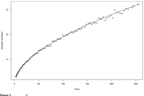
In the fig. 2 we compare σ to its estimator for several values of Nobs. We can see that our theoretical values of σ fits very well to the empirical ones.
The equation (39) gives an explicit expression of σas a product of two terms. Once the pattern and the true parameter π are fixed, the first term (Q) depends only on ᐍ and Nobs while the second one only depends on the length n of the sequence used for the parameter estima-tion (see appendix C for an explicit expression of σ in the particular case of an order 0 Markov model).
To study the variations of σ(n) as a function of n we there-fore need to study G(n) and C(n). Using equations (6) and (22) we get that
Using equations (57) and (58) in appendix A we also get that C = M + O + t EE with
M(n) = O(n2) and O(n) = O(n) (41)
so finally
for large n, with
and
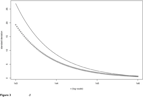
We can see on fig. 3 that is not a very good approxima-tion of σ for small n, but, as the approximation is far easier to compute (and trivial to invert) than the true value, this can be useful when we need to compute a minimum length n to obtain a given σ.
We also see on the same figure that σ grows rapidly when n decreases. For example, we get σ ⯝ 20 for n = 5000 (while equation (35) gives S ⯝ 264.4).
As we consider here a binary alphabet (k = 2) and a first order Markov model (m = 1) we have only km(k - 1) = 2 parameters to estimate with a sample of size n = 5000 (so we have 2500 sample per parameter). Although this
situ-
π =⎛ ⎝
⎜ ⎞
⎠
⎟
( )
0 3 0 7
0 6 0 4 33
. .
. .
E
S−log10P( (A− +5 1, )p ≥Nobs)=43 74285. (35)
Q p p
p N N
N N
+= − − − −
− − =
obs obs
obs obs
11 4
10 3 193 3258 36
( )
ln( ) ( , , ) .
A
A
β
(( )
a b
tG
E E
0
0 0
5 5
1 2
2 17 10 3 71 10 37
=⎡ − − ⎣
⎢ ⎤
⎦
⎥ = −⎡⎣ × − − × − ⎤⎦ ( )
( ) ( ) . .
ab ba
tG
E E
1
1 1
5 5
0 2 2 0 0 6 19 10 6 19 10 0 38
=⎡ ⎣
⎢ ⎤
⎦
⎥ =⎡ × ×
⎣ − − ⎤⎦ ( )
( ) ( ) . .
σ =Q+ tG C G× × =6 1020774.
( )
39ˆ σ
E( )n O n( ) G( )n O n
= = ⎛
⎝⎜ ⎞
⎠⎟
( )
and 1 40
σ( )n σ( )n Q A B n
= +× +
( )
42A
n t
= −
( )
→+∞
lim G C O G( ) 43
B n
n
t
= ×
( )
→+∞
lim GOG 44
ation seems quite comfortable, the sensitivity to parame-ter estimation appears in fact to be so large that we could have a factor 1040 between the true p-value and its
esti-mate.
Practical case
We have seen with our first example that our approxima-tion works very well in a simple case. Will this hold with more practical cases?
To answer this question, let us consider the following experimental design:
• one pattern: W = acgtacgt;
• two genomes: Escherichia coli K12 (ᐍ = n = 4639675) and Mycoplasma genitalium (ᐍ = n = 580076);
• five Markov orders: m = 1 to m = 5 (larger m are not con-sidered since the computation of C becomes then intrac-table).
As the sequence lengths and compositions of the two con-sidered genomes differ a lot, we have to take a different value of Nobs for each organism: Nobs = 30 for M. genital-ium and Nobs = 150 for E. coli. Proceeding as indicated in
section "simulations", we use the algorithm 1 for each experiment.
Algorithm 1 simulations for one experiment in the prac-tical case
1: estimate the order m parameter π (and μ) from the orig-inal sequence. Although these parameters are estimated, they are considered as the true parameters;
2: compute S = -log10 (N ≥ Nobs); Empirical and theoretical distributions of
Figure 1
Empirical and theoretical distributions of . A sample of size 10 000 have been used to get the empirical distribution. The solid line represents the density of (S, σ2). The adjustment test of Kolmogorov-Smirnov give D = 0.023 which
corre-sponds to a p-value of p = 5.3 × 10⁻⁵. N
obs = 1221 and n = ᐍ = 10 000. ˆ
S
ˆ
3: compute σ using approximation (23) 4: for j = 1 ... 1 000 do
5: draw a random sequence Y = Y1 ... Yn according to and order m stationary Markov model of parameter π; 6: compute N the frequency vector of all size m and size m + 1 words in Y;
7: compute Sj = S
N = -log10 (N ≥ Nobs);
8: end for
9: compute (resp. ) the mean (resp. standard devia-tion) of the sample S1,..., Sj.
We can see on table 1 the results for E. coli. For each Markov model considered, our approximation of σ is very close to the empiric ones and, as with figure 1, the Gaus-sian distribution fit well to the empiric one (data not
shown). Table 2 shows the same behaviour with M. geni-talium except for m = 5 where differs slightly more than in the other cases from its theoretical value. To understand this phenomenon, let us first recall the expression of P(N) for m = 5 using equation (15):
and as (N1 (agctac) = 0) ⯝ 2.26 × 10⁻⁶, (N
1 (gctacg) = 0) ⯝
1.35 × 10⁻¹ and (N
1 (ctacgt) = 0) ⯝ 1.24 × 10⁻⁴ we will have
P(N) = 0 roughly 14% of the time. This happened 123 times in our sample of size 1 000, each time preventing to
compute SN. The sample is hence biased and and are therefore not accurate.
What happen now if we use another statistical method to compute the pattern statistics. As the binomial approxi-mation is supposed to be close to the exact solution, we expect the standard deviation obtained with other
statisti-ˆ
S σˆ
ˆ σ
P
m
( ) ( ) ( ) ( )
( ) ( ) (
N N N N
N N
= × ×
− + × ×
1 1 1
0 0
1
agctac gctacg ctacgt
gctac
A cctacg)
ˆ
S σˆ Comparison of σ and
Figure 2
Comparison of σand . is estimated with a sample of size 1 000 and Nobs takes its values from 900 to 1 900. The solid
line represents the theoretical values and the circles the empirical ones. The statistic S is used on the x-axis. n = ᐍ = 10 000. ˆ
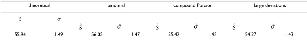
cal methods to remain close to σ. In table 3, we compare the empirical results using binomial approximations (like above) but also compound Poisson or large deviations approximations. Both empirical means and standard deviations are close to the theoretical ones thus validating the method.
Choice of a Markov model order
Through the computation of σ we can measure the sensi-tivity of pattern statistics to parameter estimations. A very natural question is then, how this variability could affect a pattern statistic study, and, as this variability grows with the Markov model order, how to choose this parameter.
Table 1: Comparison of theoretical and empirical pattern statistic mean and standard deviation on Escherichia coli K12.
m S σ
1 35.57 0.28 35.57 0.27
2 31.61 0.49 31.60 0.50
3 46.75 1.04 46.77 1.03
4 45.33 1.74 45.32 1.81
5 62.27 3.45 62.36 3.34
We consider the pattern W = acgtacgt with Nobs = 150. The sequence length is ᐍ = 4639675, we use an order m Markov model and a sample of size
M = 1 000.
ˆ
S σˆ
Comparison of σ(n) and (n) Figure 3
Comparison of σ(n) and (n). The circles reprensent σ(n) and the solid line (n). n∞ = 106 have been used to compute
the value of A and B. Nobs = 1221 and ᐍ = 10 000.
σ
We propose here to consider the case of a very simple pat-tern study: we want to find the 100 most over-represented octamers (DNA words of size 8) in a given genome. Assuming the true parameter π (and hence μ) is known, we can compute REF = {W1,..., W100}, the list of these words (ordered by decreasing statistics, so that the most over-represented one is the first one).
For each estimates and , we can compute the
100 most over-represented octamers in the genome using
the statistic and compare it to the truth. In order to do so, we first compute the true positive rate (TP rate) defined
by the rate of common words in and REF, and the rank accordance rate (RA rate) defined by the Kendall's
tau [[15], Chapter 13] between S and ranks of { ∪ REF}. Such statistic is in the range [-1,1] and has the value 1 for the complete rank accordance and the value -1 for the complete rank discordance.
As in the section "practical case", we consider two genomes: Escherichia coli K12 (ᐍ = n = 4639675) and Myc-oplasma genitalium (ᐍ = n = 580076). For each Markov model order m from 1 to 6, we estimate π on the sequence (by maximum of likelihood), compute the REF list and
then draw a sample of from which we get estimates for the expectation of TP and RA rates.
Results are given in tables 4 and 5. We can see that, sur-prisingly, the TP rate could be very low even for long genome such as E. coli when high order Markov model (m = 6) are used. Of course, these rates are even worse on M. genitalium whose genome is ten times smaller than the first one. It is also clear that the RA rate is more affected by the variability induced by parameter estimation than the TP rate.
Based on these results, we conclude that our pattern study requires a sample size per free parameter of at least a few thousands if we want reliable results. In our examples this has for consequence that the Markov order should not be greater than 4 (or 5 at the very most) for E. coli and 3 (or 4 at the very most) on M. genitalium without resulting in important errors.
Conclusion
The delta-method allows us to approximate the
distribu-tion of by a Gaussian distribudistribu-tion. This first requires to compute the expectation and covariance matrix of fre-quencies and then to study the derivative of a function which is specific of the method used to compute the pat-tern statistics. In the case of the binomial approximations, we have found an explicit expression of σ the standard deviation of .
It is clear that our approximation of σ using the delta-method relies one two major assumptions: 1) the distri-bution of N is Gaussian; 2) F+ is regular enough (e.g. not ˆ
μ πˆ REFn
ˆ
S
REFn ˆ
S REFn
REFn
ˆ
S
ˆ
S
Table 3: Comparison of theoretical and empirical pattern statistics mean and deviation on Mycoplasma genitalium.
theoretical binomial compound Poisson large deviations
S σ
55.96 1.49 56.05 1.47 55.42 1.45 54.27 1.43
We consider the pattern W = acgtacgt with Nobs = 30. The sequence length is ᐍ = 580076, we use an order m = 3 Markov model and a sample of size M = 1 000. The pattern statistics are computed (from left to right) through binomial, compound Poisson or large deviations approximations.
ˆ
S σˆ Sˆ σˆ Sˆ σˆ
Table 2: Comparison of theoretical and empirical pattern statistic mean and standard deviation on Mycoplasma genitalium.
m S σ
1 42.48 0.38 42.47 0.40
2 44.62 0.78 44.62 0.81
3 55.96 1.49 56.02 1.52
4 55.06 3.39 55.48 3.48
5 56.49 10.35 57.21* 9.09*
We consider the pattern W = acgtacgt with Nobs = 30. The sequence length is ᐍ = 580 076, we use an order m Markov model and a sample of size
M = 1 000. (*) for 123 terms in the sample we got P (N) = 0 and hence, SN was not computed.
ˆ
too steep) around E. When m grows, E closes to the boundary of the definition range of F+ hence degrading
assumption 2. Moreover, it is well known that Gaussian approximations for word frequencies become weaker when the expected numbers of their occurrences become smaller, thus degrading assumption 1. It is therefore obvi-ous that our approximation of σ will get less and less reli-able as m grows.
However, the approximation of σ has been validated through simulations and appears to be very reliable (even for m = 5 or 6). As pattern statistics computed through binomial approximations are close to the exact statistics [8], the value of σ should not differ a lot when another sta-tistical method is used. We have compared our approxi-mations to the empiric distribution obtained using compound Poisson and large deviations approximations and, as expected, our approximations remains quite relia-ble even for these statistical methods.
The variability due to parameter estimation is of course related to the Markov model order m and to the size k of the alphabet (as we have km+1 parameters for this model)
and to the length n of the sequence used for this estima-tion. For example, considering an order m = 6 model with n = 4639675 (Escherichia coli K12 complete genome) requires to estimate 3 × 46 = 4096 free parameters which
results roughly in 400 observation per free parameter. Although this situation seems quite comfortable, we have seen with our simulations that it leads an unacceptable variability for pattern statistics.
As literature often advices to use the highest possible Markov order for a given pattern problem (which means m = h - 2 for pattern of size h) it is easy to understand that such a practice could have very detrimental effects on the
computed statistics unless huge data are available for esti-mation purpose. Even if we consider the more reasonable attitude to choose m using the classical framework of model selection (e.g. using the Akaike Information Crite-rion – AIC –) we get m = 5 for Mycoplasma genitalium and m = 6 for Escherichia coli K12 hence resulting in both cases in the same catastrophic results in terms of false positive and even worse ones in terms of ranking.
Moreover, we assumed here that our model was homoge-neous all along the considered sequences. This is obvi-ously completely false when complete genomes are considered. So it is more likely that the sample size n would be far smaller than a million on classical pattern studies (even of human genomes for example). As a result, the variability we pointed out in this paper will have a considerable detrimental effect on most studies unless the Markov order is carefully set.
In order to do so, we advice to compute our approxima-tion of σ each time a pattern statistic is produced and then to evaluate, either by simulation (like in this paper) or by a theoretical work the impact of this variability on the considered study.
Competing interests
The author declares that he has no competing interests.
Appendix A
We give here the expression of the covariance matrix C introduced in section "distribution of N = (N0, N1)". The sequence Y (of length n) is generated by an homogeneous, stationary and ergodic order m Markov model of parame-ter π and stationary distribution μ. We want to compute the covariance of the vector N of random frequencies of size m and m + 1 words.
Table 5: Mean true positive rate and rank accordance rate in Mycoplasma genitalium.
Markov order 1 2 3 4 5 6
TP rate 95.5% 93.6% 90.4% 81.8% 66.0% 25.0%
RA rate 92.6% 85.4% 79.8% 66.5% 45.1% 11.0%
× 103 48.33 12.08 3.02 0.76 0.19 0.05
Both quantities are estimated with 1 000 simulations. We consider the 1 00 most over-represented octamers, the sequence length is ᐍ = 580076. The last row gives the sample size per free parameter (length n of the sequence divided by the number km(k - 1) of parameters).
Table 4: Mean true positive rate and rank accordance rate in Escherichia coli K12.
Markov order 1 2 3 4 5 6
TP rate 99.0% 98.0% 97.9% 94.4% 82.1% 47.6%
RA rate 99.0% 95.5% 91.5% 83.9% 68.0% 36.5%
× 103 383.33 95.83 23.96 5.99 1.50 0.37
For any word w (of size hw), we introduce the following notation for hw ≤ i ≤ n
where = Yi ... Yj for all i ≤ j. If hw ≥ m, we denote by
the probability to see one occurrence of w at a given posi-tion in the sequence. At last, if we consider another word v (of size hv = m) and if hw = m, we denote by
the probability to see occurrences of v and w separated by a gap of length δ.
For any words v an w (to simplify, we suppose that hv ≥ hw) then, for all δ∈ and
max(hv, hw - δ) ≤ i ≤ min(n, n - δ) we have
[Ii (v) Ii+δ (w)] = Dδ (v, w) (48)
which do not depend on i.
It is therefore easy to show that
where the main part (2n - hv - hw + 2 terms) is given by
and the overlapping part (hv + hw - 1 terms) by
and with
As we have
C(v, w) = M (v, w) + O (v, w) - E (v) E (w) (55)
the problem is hence to compute M and O for all pairs of size m or m + 1 words. In order to simplify, we will just treat here the case of a pair of size m words (other cases can be derived from this special case).
For the main part we obtain
(2n - 2m + 2 terms). As Pk (v, w) quickly converges toward
μ(w) when k grows (convergence speed is given by λk where λ is the magnitude of the second eigenvalue of the transition matrix Π). So there exists a rank r ≥ m such as
which has only 2r - 2m + 1 terms.
And for the overlapping part we get
which has 2m + 1 terms.
So the overall complexity for the computation of one term of C is hence O(r) where the value of r is directly con-nected to the magnitude λ of the second eigenvalue of the transition matrix.
I wi w i Y w
i hwi
( )= { }= { } ( )
− + = I end in position I
1 45
Yij
p w wm wm wm whh m wh w
( )=μ( 1) (Π 1, +1)... (Π −1− , ) (46)
Πδ
δ
( , )v w p vxw( ) ( )
x = ∈
∑
47 Z EE[ ( ) ( )] ( , )
( , )
N vN w D v w
N D v w
h i n i i h n h n n h w v w =
( )
= = − − = = − −∑
∑
δ δ δ δ δ 49 vvv w v m
∑
( )
= +
( )
50
51 M( , ) O( , )
M( , )v w N D ( , )v w N D v w( , ) ( )
h n h h n h v w w v = − − + = − = −
∑
δ δ∑
δ δ δ δ 52O( , )v w N D v w( , ) ( )
h h v w = =− + −
∑
δ δ δ 1 1 53 Nn h h n h h
n h h h
n h n h
w w w v
v w v
v δ δ δ δ δ δ = − + + ∈ − − − + ∈ − − + − ∈ − 1 1 0 1 0 [ , [ [ , ]
] , vv]
( ) ⎧ ⎨ ⎪ ⎩ ⎪ 54
M( , ) ( ) ( , )
( ) ( , )
(
v w N w w v
N v v w
m m n m m m n m = + − − + = − − + = −
∑
∑
δ δ δ δ δ δ μ μ Π Π 1 1 5 56)M( , ) ( ) ( ) ( )
( ) ( , )
v w v w N N
N w w v
N r n m m m r μ μ μ δ δ δ δ δ δ − = − − − + = − + + +
∑
∑
Π 11
δδ δ
δ μ
( )v m ( , )v w ( ) m r Π − + = −
∑
1 1 57O( , ) ( )
( )
{ }
v w N v
N p wv
v w m
m m
vm wm
= × × + × × = − = − − +
{
=∑
− + 0 1 1 1 1 1 μ δ δ δ δ II δ
}}
− + = − =
{
}
+∑
× × + − N p vwmmm
vm wm
δ δ
δ δ δ
( 1) ( )
1 1
1 1
In the particular case of an order one Markov model (m = 1), we give here the complete expressions of M and O.
For all a, b, c, d ∈ , we have
O (a, b) = nμ(a) {a = b} (60)
With the example given in section "validation" we get for the expectation
= [4615.4 5384.6] (65)
and
= [1384.5 3230.4 3230.4 2153.6] (66)
The magnitude of the second eigenvalue of Π is λ = 0.3, then rank r = 19 give a relative error < 10 -10 and we get for
the covariance
and
Appendix B
The beta function is defined by
for all a, b > 0. The incomplete beta function for all x ∈ [0,1] is then defined by
and
Using a continued fraction representation, these functions
can be quickly numerically evaluated in O( )
in the worst case [15, Chapter 6].
A great interest of this function is that it is connected to the cumulative distribution function of a binomial distri-bution by the following relation:
with (n, k) ∈ * × , 0 ≤ k ≤ n and p ∈ [0,1].
Finally, let us remark that the incomplete beta function is differentiable in x and that
Appendix C
We give here the complete expression of σ for a single pat-tern in the special case of an order m = 0 homogeneous Markov model of parameter μ.
The MLE of μ is given by
where N1 is the frequency of all letters.
M( , ) ( )( ) ( ) ( )
( ) ( ) ( , ) ( ) ( , )
a b n r n r a b
n b b a a a b
− + −
+ −
(
+)
1 μ μ
δ μ Πδ μ Πδ ((59)
1 1 δ = −
∑
r IM( , )
( , ) ( )( ) ( ) ( )
( ) ( ) ( , ) ( )
ab c
a b n r n r a c
n c c a a
Π Π − − − + − − + 1 1 μ μ δ μ δ μ ΠΠδ δ
( , )b c ( )
r
(
)
= −∑
61 1 1O( , )
( , ) ( ) ( )({ } { }) ( )
ab c
a b n a a c b c
Π = −1μ I = +I = 62
M( , )
( , ) ( , ) ( )( ) ( ) ( )
( ) ( ) (
ab cd
a b c d n r n r a c
n c Π Π Π − − − − + − − 1 2 2 μ μ
δ μ δ dd a a b c r , )+ ( ) ( , ) ( )
(
)
= −∑
μ δ δ Π 63 1 1O( , )
( , ) ( ) ( )
( ) ( , ) ( ) (
{ }
{ }
ab cd
a b n a
n c d c a
ab cd a d Π Π = − + − + = = 1 2 μ μ μ I
I ))I{b c=} ( )
(
)
64E0t
E1t
C0 0 1338 28 1338 28
1338 28 1338 28 67
, . . . . ( ) = − − ⎡ ⎣ ⎢ ⎤ ⎦ ⎥
C1 0
1146 9 191 2 191 2 1529 2
1146 9 191 2 191 2 1529 2
, . . . . . . . . = − − − − ⎡ ⎣
⎢ ⎤⎦⎥⎥ (68)
C11
1536 8 390 0 390 0 756 9
390 0 581 2 581 0 772 2
390 0 5
, . . . . . . . . . = − − − − −
− 881 0 581 2 772 2
756 9 772 2 772 2 2301 4
69 . . . . . . . ( ) − − − − ⎡ ⎣ ⎢ ⎢ ⎢ ⎢ ⎢ ⎤ ⎦ ⎥ ⎥ ⎥ ⎥ ⎥
β( , )a b =
∫
ta−1( −t)b−1dt ( ) 01
1 70
β( , , )x a b =
∫
xta−1( −t)b− dt ( ) 0 1 1 71 β− β β − − = −( )
=∫
−( )
( , , ) ( , ) ( , , ) ( )x a b a b x a b
ta t dt
x b 72 1 73 1 1 1
max( , )a b
P( ( , ) ) ( , , )
( , ) ( )
n p k p k n k k n k
≥ = − + − + β β 1 1 74 ∂β ∂ ( , , ) ( ) ( )
x a b
x x x
a b
= −11− −1 75
μN
N
= 1 76
Publish with BioMed Central and every scientist can read your work free of charge "BioMed Central will be the most significant development for disseminating the results of biomedical researc h in our lifetime."
Sir Paul Nurse, Cancer Research UK
Your research papers will be:
available free of charge to the entire biomedical community
peer reviewed and published immediately upon acceptance
cited in PubMed and archived on PubMed Central
yours — you keep the copyright
Submit your manuscript here:
http://www.biomedcentral.com/info/publishing_adv.asp
BioMedcentral A Gaussian approximation gives
(N1) ⯝ (E1, C1,1) (77)
with E1 = nμ and, for all a, b ∈ ,
C1,1 (a, b) = nμ (a) a = b - nμ(a) × nμ(b) (78) We have also
which implies for all a ∈ that
So finally we get
where Q is either defined by equation (24) if the pattern is over-represented or by equation (28) if under-repre-sented.
References
1. Atteson W: Calculating the exact probability of language-like patterns in biomolecular sequences. Pro 6th Int Conf on Intelligent Systems for Molecular Biology 1998:17-24.
2. Régnier M, Szpankowski W: On pattern frequency occurrences in a Markovian sequence. Algorithmica 1998, 22(4):631-649. 3. Robin S, Daudin JJ: Exact distribution of word occurrences in a
random sequence of letters. J App Prob 1999, 36:179-193. 4. Nuel G: Effective p-value computations using Finite Markov
Chain Imbedding (FMCI): application to local score and to pattern statistics. Algorithms Mol Biol 2006, 1(1):5.
5. Kleffe J, Borodovski M: First and second moment of counts of words in random text generated by Markov chains. Comp Applic Biosci 1992, 8:443-441.
6. Prum B, Rodolphe F, de Turckheim E: Finding words with unex-pected frequencies in DNA sequences. J R Statist Soc B 1995, 11:190-192.
7. van Helden J, André B, Collado-Vides J: Extracting Regulatory Sites from the Upstream Region of Yeast Genes by Compu-tational Analysis of Oligonucleotide Frequencies. J Mol Biol 1998, 281:827-842.
8. Nuel G: S-SPatt: Simple Statististics for Patterns on Markov chains. Bioinformatics 2005, 21(13):3051-3052.
9. Chrysaphinou O, Papastavridis S: A limit theorem on the number of overlapping appearances of a pattern in a sequence of independent trials. Proba Theory Relat Fields 1988, 79(1):129-143. 10. Arratia R, Goldstein L, Gordon L: Poisson approximation and the
Chen-Stein method. Stat Sci 1990, 5(4):403-434.
11. Schbath S: Compound Poisson approximation of word counts in DNA sequences. ESAIM Probab Stat 1995, 1:1-16.
12. Nuel G: LD-SPatt: Large Deviations Statistics for Patterns on Markov Chains. J Comput Biol 2004, 11(6):1023-1033.
13. Oehlert GW: A note on the delta method. American Statistician 1992, 46:27-29.
14. Reinert G, Schbath S, Waterman M: Chapter 6: Statistics on words with applications to biological sequences. In Applied Combinatorics on Words Cambridge Universtity Press; 2005. 15. Press WH, Teukolsky SA, Vetterling WT, Flannery BP: Numerical
Rec-ipes in C 2nd edition. Cambridge Universtity Press; 1988.
L
I
P
nh a
A a
a
( )N = N ( ) ( ) ( )
∈
∏
179
1 1
∂
∂ = ×
P a
A a a P
a ( )
( )
( )
( ) ( ) ( )
( )
N
N N N
G 1
1
1
1
80
N