Optimal Sequential Sampling Plans
Using Dynamic Programming Approach
Mohammad Saber Fallah Nezhad
Industrial Engineering Department, Yazd University, Yazd, Iran [email protected]
Abolghasem Yousefi Babadi
MS Student of Industrial Engineering, Yazd University, Yazd, Iran [email protected]
Minoo Momeni
MS Student of Industrial Engineering, Yazd University, Yazd, Iran [email protected]
Noushin Sayani
MS Student of Industrial Engineering, Yazd University, Yazd, Iran [email protected]
Fatemeh Akhoondi
MS Student of Industrial Engineering, Yazd University, Yazd, Iran [email protected]
Abstract
In this paper we proposed a dynamic programming procedure to develop an optimal sequential sampling plan. A suitable cost model is employed for depicting the cost of sampling, accepting or rejecting the lot. This model is based on sequential approach. A sequential iterative approach is used for modeling the cost of different decisions in each stage. In addition a backward recursive algorithm is developed to solve the dynamic programming. On the other hand, the purpose of this paper is to introduce a new sequential acceptance sampling plan based on dynamic programming. At the end of this paper a numerical example is solved to show how this model works and then sensitivity analyses of main parameters of acceptance sampling model are carried out.
Keywords: Sampling Plan; Dynamic Programming; Optimization; Recursive Approach.
1. Introduction
Acceptance sampling is a useful tool which is used in quality control in order to design decision principles for lot acceptance problem. Depending on number of defective items in sample, the decision may be,
1. Accepting the batch 2. Rejecting the batch
3. Continuing the sampling and repeating decision process.
Therefore we expect to have less defective items in accepted batches using this approach. This method encourages mangers to use it for two reasons:
2. Having reverse relevance between quality level and inspections required (Montgomery 2005).
We use sampling plans usually when we have destructive inspection experiments or cost of 100% inspecting is high or it takes long time. In this work a new decision making approach for accepting or rejecting a sample based on recursive inference is improved. Recursive inference is used for determining the optimal decision. Also when none of the decisions of accepting or rejecting is optimal, it is assumed that we can have more observations and continue to the next stage. Thus a mathematical model is developed which is optimal solution because of using stochastic dynamic programming approach. The main objective of model is to optimize cost of sampling system based on fraction of defective items. On the other hand Sequential sampling reduces the number of samples required to evaluate a population level by 40-80% in comparison with classical sampling techniques (Boivin and Vincent 1983).
Sequential sampling plans are designed to enhance the performance of sampling methods. First step of this method is to inspect an initial sample from the lot then we decide to accept, reject the lot or take another sample by analyzing the results of inspected sample. Sequential sampling plans are often applied where minimizing sample size is very important (Montgomery 2005). In such plans, item are inspected successively in different stages, until a decision is made on the lot or process thus the sample size of this method is not determined until the lot is accepted or rejected. Sequential sampling plans select the suitable decision quickly, especially when quality is particularly good or particularly.
2. Literature Review
The purpose of sampling plans is to provide users with evidence that the items reach the quality levels required and agreed upon. Sampling plans has been commonly conducted by quality inspection for acceptance purposes, which is based on the statistical theory. Acceptance sampling inspection is a statistical tool concerned with sampled items to make a decision about inspected products; especially to check whether items have met pre agreed quality specifications. Sampling inspection process concern with the definition of quality characteristics, sample size, acceptance criteria, and a combination of quality levels required by the producer and the consumer (Tong et al 2011).
Golub (1953) presented a method for determining optimal Sampling inspection plans based on the criterion of minimizing sums of both producer’s and consumer’s risks when sample size is fixed. Duarte and Saraiva (2008) proposed an optimization approach for designing acceptance sampling plans by combining quality levels required by the producer and the consumer when the fraction of nonconformities being modeled by a Poisson probability distribution function. Sadeghpour-Gildeh et al. (2008) proposed an acceptance double sampling plan when the fraction of defective items is assumed to be a fuzzy number. Jamkhaneh et al. (2009) further developed an acceptance single sampling plan when the proportion of nonconforming items follows a fuzzy Poisson distribution.
appropriate distribution to describe the random fluctuation involved in an Acceptance sampling (Latha and Jeyabharathi 2012). Niaki and Fallahnezhad (2009) used both the stochastic dynamic programming and Bayesian inferences concept to design sampling plan. Fallahnezhad and Hosseininasab (2011) proposed an acceptance sampling plan bases on cost objective function. Fallahnezhad and Niaki (2012) proposed an acceptance sampling plan based on number of successive conforming items. Fallahnezhad et al (2011) proposed an acceptance sampling plans based on the cumulative sum of the number of successive conforming items. Also Fallahnezhad et al (2012) proposed Bayesian acceptance sampling plan based on the cost function. Aslam et al. (2012) presented a decision rule for repetitive acceptance sampling plan. Fallahnezhad (2012) analyzed the acceptance sampling design with minimum angle method. Fallahnezhad and yousefi (2014) developed a decision tree for designing an optimal acceptance sampling plan based on cost objective function in the presence of inspection errors. They used Bayesian inference to obtain required probabilities. Then the optimal decisions are determined using a backward recursive approach. They have shown that acceptance sampling model based on Bayesian inference is efficient and less expensive than the single sampling plan. Fallahnezhad and Aslam (2013) proposed a decision tree for optimizing the cost acceptance sampling problem based on recursive modeling.
Tagaras (1998) studied the joint process control and machine maintenance problem of a Markovian deteriorating machine. He assumed that sampling and preventive maintenance were performed at fixed intervals. Kuo (2006) developed an optimal adaptive control policy for joint machine maintenance and product quality control. He included the interactions between the machine maintenance and the product sampling in the search for the best machine maintenance and quality control strategy for a Markovian deteriorating batch production system. Wortham and Wilson (1971) proposed a backward recursive technique for optimal sequential sampling plans.
Most attempts to minimize sampling cost were concentrated on reducing expected sample size and reducing inspection cost. But the costs associated with the accept-reject decisions should be considered in designing the sampling plans. The cost of each defective item in an accepted lot can be evaluated very accurately in some quality control environments. On the other hand, cost of accepting defective item can be estimated by considering its results in practical situations. Cost estimates for rejected lots are readily obtained by considering the rectification method (Wortham and Wilson 1971).
In this research, a new model for acceptance sampling problem is introduced. The objective of the model is to determine the optimal decision that minimizes the total cost including the cost of rejecting the batch, the cost of inspection and the cost of defective items.
The assumptions and notations of the proposed method are presented in section 3, the model is presented in section 4 and the solution algorithm along with numerical demonstration on the application comes in section 5, sensitivity analyses are performed in Section 6 and we discussed and conclude the results in Section 6.
3. Dynamic Modeling
Following notations are used in the rest of paper,
N: Lot size
n: accumulated number of items sampled
m: maximum number of items allowed to sample
x: accumulated number of defective items observed in the n items sampled
X: number of defective items in the lot
y = X - x: number of defective items remaining in the N- n items of lot that has not been sampled
E(y|x):expected number of defective items in the part of the lot that has not been sampled
p: proportion of defective items in the lot
cs: cost of sampling and inspecting one item
cr: cost of replacing, reworking or repairing a defective item
ca: cost of one defective item in an accepted lot.
Assume there is a batch with N items. A sample of n items is selected. Each defective item is replaced with a good one in sample after inspection. We although call “m” equal
to the maximum number of items that can be inspected and it is determined by economic considerations. Based on inspection's output we want to make an optimal decision. The possible decisions are as follows,
Rejecting the lot
accepting the lot
Taking another sample
4. Sampling Plan Using Dynamic Programming
Let K (n,x) be the expected cost of accepting the lot after observing x defective items in a n sampled items thus we have
a s r a
K (n,x) = c n + c x + c E(y|x) Where;
csn: is accumulated number of items sampled (n) multiplied by cost of sampling and inspecting one item (cs), so this item is total cost of inspecting the items in sample.
crx: is accumulated number of defective items sampled (x) multiplied by cost of replacing, reworking or repairing a defective item (cr), so this item is total cost of replacing, reworking or repairing defective items.
caE(y|x): is expected number of defective items in the part of the lot that has not been sampled (E(y|x)) multiplied by cost of one defective item in an accepted lot (ca), thus this item is total cost of defective items in an accepted lot.
And now let K (n,x) be the expected cost of rejecting the lot after observing r x defective items in n sampled items thus we obtain
r s r r
K (n,x) = c N + c x + c E(y|x)
Where;
csN: is Lot size (N) multiplied by cost of sampling and inspecting one item (cs), so this item is total cost of inspecting the lot after rejecting the batch.
crx: is accumulated number of defective items sampled (x) multiplied by cost of replacing, reworking or repairing a defective item (cr), so this item is total cost of replacing, reworking or repairing defective items.
crE(y|x): is expected number of defective items in the part of the lot that has not been sampled (E(y|x)) multiplied by cost of replacing, reworking or repairing a defective item (cr), so this item is total cost of replacing, reworking or repairing defective items in the part of the lot that has not been sampled.
Let K (n,x) denotes the cost of taking one more sample after observing s x defective items
in n sampled items. If *
K (n,x) denotes the optimal cost of decision making system, thus following is concluded,
*
a r s
K (n,x) = Min { K (n,x) , K (n,x) , K (n,x)} where,
*
a r
K (m,x) = Min { K (m,x) , K (m,x)}
It is obvious that in decision of taking one more sample, if the item was not defective then we move to state (n+1,x) which its optimal cost is equal to *
equal toK (n+1,x+1) . Since the expected value of the proportion of defective items is * E(p) thus using the conditional mean formula, following result is concluded,
* *
* *s
K (n,x) =E K (n+1,x) (1-p) + K (n+1,x+1) p =K (n+1,x) (1-E(p)) + K (n+1,x+1) E(p)
Also it is obvious that E(p)obtained as follows, x
E(p)= n
And E(y|x) obtained as follows
Nx E(p)=N× E(p) - x=
n
N n x x
n
5. Numerical Example
Assume a lot of N 250 items is received, the maximum sample size ism25, the cost of each inspection is cs 0.2, the cost of accepting a nonconforming item is ca 2.5, and the cost of replacing, reworking or repairing a defective itemcr 1.5. Moreover, assume x=3 out of n=20 inspected items are nonconforming. Thus following results are concluded,
E(p)=0.15
E(y|x) N× E(p) - x = 250×0.15 - 3 = 34.5
Thus following results are obtained,
a
r
* *
s *
a r s
K (20,3) = 0.2×20 + 1.5×3 + 2.5×34.5= 90.75
K (20,3) = 0.2×250 + 1.5×3 + 1.5×34.5= 102.25
K (20,3) = K (21,3) (0.85) + K (21,4) (0.15)
K (20,3) = Min { K (20,3) , K (20,3) , K (20,3)}
Now to evaluate the value of *
K (20,3) , first we need to determine the values of
* *
K (21,3) , K (21,4) . The value of K (21,3) is determined as following, *
a
r
* s
*
a r s
E(y|x) =N× E(p) - x = 250× - 3 =
K (21,3) =
K (21,3) =
K (21,3) = K (22,3)(0.857143)+ K*(22,4)( )
K (21,3) = M
0.142857 32.71429
86.28571
99.3
in { K (21,3) , K (21,3) , 7143
K 0
(
.142857
Now to evaluate the value of K (21,3) , first we need to determine the values of *
* *
K (22,3), K (22,4) . The value of K (22,3) is determined as follows, *
a
r
* *
s *
a r s
E(y|x) =
K (22,3) =
K (22,3) =
K (22,3) = K (23,3)(0.863636) + K (23,4)( )
K (22,3) = Min { K 31.
(22 09091
82.22727
96.73636
0.136
,3) , K (22,3
36
) , K (
4
22,3)}
Now to evaluate the value ofK (22,3) , first we need to determine the values of*
* *
K (23,3), K (23,4) . And then we need K (24,3), K (24,4) , K (25,3) , K (25,4) . * * * *
Since in states(25,3), (25,4) , we reach the end of decision making horizon, therefore the
values of K (25,3),K (25,4) are obtained as follows, * *
*
a r
a
r *
a r
E(y|x) =27
Ka(25,3) = 72
Kr(25,3) = 90
K (25,3) = Min { K (25,3) , K (25,3)}= 72
E(y|x) = 36
K (25,4) = 96
K (25,4) = 105
K (25,4) = Min { K (25,4) , K (25,4)}= 96
Thus K (24,3) can be obtained, *
a r
*
s
75.125 92.0
K (24,3)= , K (24,3)= ,
K (24,3) = Min =75
K (24,3)=72 (0.875) + 96(0.125) 75
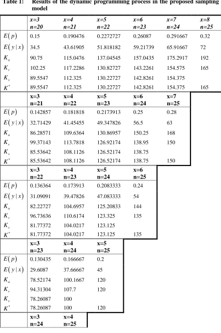
Table 1: Results of the dynamic programming process in the proposed sampling model
x=3 x=4 x=5 x=6 x=7 x=8
n=20 n=21 n=22 n=23 n=24 n=25
E p 0.15 0.190476 0.2272727 0.26087 0.291667 0.32
|
E y x 34.5 43.61905 51.818182 59.21739 65.91667 72
a
K 90.75 115.0476 137.04545 157.0435 175.2917 192
r
K 102.25 117.2286 130.82727 143.2261 154.575 165
s
K 89.5547 112.325 130.22727 142.8261 154.375
*
K 89.5547 112.325 130.22727 142.8261 154.375 165
x=3 x=4 x=5 x=6 x=7
n=21 n=22 n=23 n=24 n=25
E p 0.142857 0.181818 0.2173913 0.25 0.28
|
E y x 32.71429 41.45455 49.347826 56.5 63
a
K 86.28571 109.6364 130.86957 150.25 168
r
K 99.37143 113.7818 126.92174 138.95 150
s
K 85.53642 108.1126 126.52174 138.75
*
K 85.53642 108.1126 126.52174 138.75 150
x=3 x=4 x=5 x=6
n=22 n=23 n=24 n=25
E p 0.136364 0.173913 0.2083333 0.24
|
E y x 31.09091 39.47826 47.083333 54
a
K 82.22727 104.6957 125.20833 144
r
K 96.73636 110.6174 123.325 135
s
K 81.77372 104.0217 123.125
*
K 81.77372 104.0217 123.125 135
x=3 x=4 x=5
n=23 n=24 n=25
E p 0.130435 0.166667 0.2
|
E y x 29.6087 37.66667 45
a
K 78.52174 100.1667 120
r
K 94.31304 107.7 120
s
K 78.26087 100
*
K 78.26087 100 120
E p 0.125 0.16
|
E y x 28.25 36
a
K 75.125 96
r
K 92.075 105
s
K 75
*
K 75 96
x=3 n=25
E p 0.12
|
E y x 27
a
K 72
r
K 90
s K
*
K 72
The recursive approach of solving proposed dynamic programming model is summarized in the above Table. It is seen that the model can be easily solved using a computer program. In the next section, sensitivity analysis is performed on different parameters.
6. Sensitivity Analysis
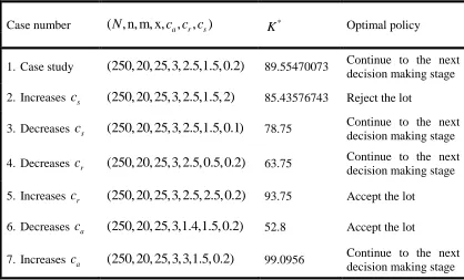
A sensitivity analysis is performed on the parameters of the problem and the results are summarized in the Table (2).
Table 2: Optimal solution for different values of parameters
Case number ( , n, m, x,N c c ca, , )r s *
K Optimal policy
1. Case study (250, 20, 25,3, 2.5,1.5, 0.2) 89.55470073 Continue to the next decision making stage
2. Increases cs (250, 20, 25,3, 2.5,1.5, 2) 85.43576743 Reject the lot
3. Decreases cs (250, 20, 25,3, 2.5,1.5, 0.1) 78.75 Continue to the next decision making stage
4. Decreases cr (250, 20, 25,3, 2.5, 0.5, 0.2) 63.75 Continue to the next decision making stage
5. Increases cr (250, 20, 25,3, 2.5, 2.5, 0.2) 93.75 Accept the lot
6. Decreases ca (250, 20, 25,3,1.4,1.5, 0.2) 52.8 Accept the lot
The results are summarized as follows,
By comparing case one and case two, it is seen that when the cost of sampling and inspecting one item
cs increases, then the optimal decision in the proposed method isto reject the lot. By comparing case one and case three, it is seen that when the cost of sampling and inspecting one item
cs decreases, then the optimal decision in theproposed method is to continue to the next decision making stage. So it is logical, because when the cost of inspecting the one item decreases then, optimal policy would be to inspect more items.
Also it is seen that when the cost of replacing, reworking or repairing a defective item
cr increases, then the optimal decision in the proposed method is to accept the lot asexpected. Also when the cost of replacing, reworking or repairing a defective item
crdecreases, then the optimal decision in the proposed method is to continue to the next decision making stage.
It is seen that when the cost of accepting a nonconforming item
ca decreases, then the optimal decision in the proposed method is to accept the lot. Since decreasing cost of accepting a nonconforming item leads to decrease the cost of accepting the lot thus optimality of the acceptance decision is logical. Also it is seen that when the cost of accepting a nonconforming item
ca increases, then the optimal decision in theproposed method is to continue to the next decision making stage.
7. Conclusion
This paper presents a dynamic programming procedure to design an optimal sequential sampling plan. That is very important for quality control managers to have a good lot with minimum cost. Since the cost of inspecting all items is very high, it is popular that managers use sampling for this purpose. In this work, a new decision making approach for accepting or rejecting a sample based on recursive inference is improved. The objective of the model is to determine the optimal decision that minimizes the total cost including the cost of rejecting the batch, the cost of inspection and the cost of defective items. Also when none of the decisions of accepting or rejecting is optimal, it is assumed that we can have more observations and continue to the next stage. A mathematical model is developed which leads to optimal solution because of using dynamic programming approach. Also, sequential approach is used for obtaining the cost of different decisions in each stage. A numerical example is solved to elaborate the application of the proposed methodology. At the end sensitivity analyses of main parameters are performed and the results are discussed.
References
1. Montgomery, D., (2005). Introduction to Statistical Quality Control. fifth ed., John Wiley & Sons Inc., New York.
3. Golub, A. (1953). Designing single-sampling inspection plans when the sample size is fixed. Journal of the American Statistical Association 48 (262), 278–288.
4. Duarte, B.P.M., Saraiva, P.M. (2008). An optimization-based approach for designing attribute acceptance sampling plans. International Journal of Quality & Reliability Management 25 (8), 824–841.
5. Sadeghpour-Gildeh, B., Yari, G. & Jamkhaneh, E.B. (2008). Acceptance double sampling plan with fuzzy parameter. Proceeding of the 11th Joint Conference on Information Sciences, Shenzhen, China, Atlantis Press, France.
6. Jamkhaneh, E.B., Gildeh, B.S. & Yari, G.H. (2009). Acceptance single sampling plan with fuzzy parameter with the using of Poisson distribution. World Academy of Science, Engineering and Technology, 49, 1017–1021.
7. Latha, M., Jeyabharathi, S. (2012). Selection of Bayesian Chain Sampling Attributes Plans Based On Geometric Distribution. International Journal of Scientific and Research Publications, 2(7), 1-8.
8. Niaki, S.T.A., Fallahnezhad, M.S. (2009). Designing an Optimum Acceptance Plan Using Bayesian Inference and Stochastic Dynamic Programming. International Journal of Science and Technology (Scientia Iranica), 16(1), 19-25.
9. Fallahnezhad, M.S., Hosseininasab, H. (2011). Designing a Single Stage Acceptance Sampling Plan based on the control Threshold policy. International Journal of Industrial Engineering & Production Research, 22(3), 143-150.
10. Fallahnezhad, M.S., Niaki, S.T.A. (2012). A New Acceptance Sampling Policy Based on Number of Successive Conforming Items. To Appear in Communications in Statistics-Theory and Methods.
11. Fallahnezhad, M.S., Niaki, S.T.A. & Abooie, M.H. (2011). A New Acceptance Sampling Plan Based on Cumulative Sums of Conforming Run-Lengths. Journal of Industrial and Systems Engineering, 4(4), 256-264.
12. Fallahnezhad M.S, Yousefi Babadi A. (2014). A New Acceptance Sampling Plan Using Bayesian approach in the presence of inspection errors. Transactions of the Institute of Measurement and Control; 1–14.
13. Fallahnezhad M.S, Aslam M. (2013). A new economical design of acceptance sampling models using Bayesian inference. Accreditation and Quality Assurance; 18: 187-195.
14. Fallahnezhad, M.S., Niaki, S.T.A. & Vahdat, M.A. (2012). A New Acceptance Sampling Design Using Bayesian Modeling and Backwards Induction. International Journal of Engineering, 25(1), 45-54.
15. Aslam, M., Niaki, S.T.A., Rasool, M. & Fallahnezhad, M.S. (2012). Decision Rule of Repetitive Acceptance Sampling Plans Assuring Percentile Life. Scientia Iranica, Transactions E, 19(3), 879-884.
17. Kuo, Y. (2006). Optimal adaptive control policy for joint machine maintenance and product quality control. European Journal of Operational Research, 171, 586–597.
18. Tagaras, G. (1988). Integrated cost model for the joint optimization of process control and maintenance. Journal of Operational Research Society, 39, 757–766.
19. Wortham, A.W., Wilson, E.B.A. (1971). Backward recursive technique for optimal sequential sampling plans. Naval Research Logistics Quarterly, 18, 203-213.