Advanced Manufacturing Technologies:
Data Envelopment Analysis with Double Frontiers”
Hossein Azizi
Department of Applied Mathematics
Parsabad Moghan Branch, Islamic Azad University Parsabad Moghan, Iran
hazizi@iaupmogan.ac.ir
Recently, using the data envelopment analysis (DEA) with double frontiers approach, Wang and Chin (2009) proposed a new approach for the selection of advanced manufacturing technologies: DEA with double frontiers and a new measure for the selection of the best advanced manufacturing technologies (AMTs). In this note, we show that their proposed overall performance measure for the selection of the best AMT has an additional computational burden. Moreover, we propose a new measure for developing a complete ranking of AMTs. Numerical examples are examined using the proposed measure to show its simplicity and usefulness in the AMT selection and justification.
Keywords: Data envelopment analysis; Advanced manufacturing technology; Optimistic and pessimistic efficiencies.
1. Introduction
Selection of advanced manufacturing technologies (AMTs) is an important decision-making process for the explanation and implementation of AMTs. This requires careful consideration of various performance criteria (Wang & Chin, 2009). As an excellent method for performance evaluation based on data when a set of decision-making units (DMUs) has multiple inputs and outputs, data envelopment analysis (DEA) has proven its value. Therefore, the DEA has been widely used for AMT selection and justification.
For best use of the DEA, Wang and Chin (2009) introduced a new DEA method called “DEA with double frontiers” for AMTs selection and justification. The DEA with double frontiers considers two different efficiencies, i.e. optimistic and pessimistic efficiencies for decision-making. In this note, we show that the overall performance measure proposed by Wang and Chin (2009) for selecting the best AMT has an additional computational burden and may affect the ranking results. Finally, we propose a new measure to develop a complete ranking of AMTs.
2. DEA with double frontiers
2.1. Review on Wang and Chin’s (2009) work
Assume that there are n AMTs for selection that must be evaluated in terms of m inputs and s outputs. For AM Tj ( j1,,n), we show input values with xij (i1,,m) and
output values with yrj (r 1,,s), all of which are known and non-negative. The
optimistic efficiency of AM Tj compared to other AMTs is measured with the following
CCR model (Charnes et al., 1978):
. , , 1 ; , , 1 , 0 , , 1 , , , 1 , 0 s.t. max 1 1 1 1 m i s r v u x v n j x v y u y u i r m
i i io
m
i i ij
s
r r rj
s
r r ro
o
(1)where AMT is the AMT under evaluation, and o ur (r1,,s) and vi (i1,,m)
are decision variables. If there is a set of positive weights u*r (r 1,,s) and vi*
(i1,,m) to supply o* 1, then AMT is called optimistic efficient; otherwise, it is o
called optimistic non-efficient.
In addition, the pessimistic efficiency of AMT compared to other AMTs can be o measured with the following model (Azizi & Wang, 2013; Liu & Chen, 2009; Wang et al., 2007): . , , 1 ; , , 1 , 0 , , 1 , , , 1 , 0 s.t. min 1 1 1 1 m i s r v u x v n j x v y u y u i r m
i i io
m
i i ij
s
r r rj
s
r r ro
o
(2)When there is a set of positive weights ur* (r 1,,s) and vi* (i1,,m) to supply
1 *
o
, then AMT is called pessimistic inefficient; otherwise, it is called pessimistic o non-inefficient.
Optimistic and pessimistic efficiencies are measured from different perspectives, and often lead to two different rankings for AMTs. Therefore, an overall performance measure is needed to obtain a single overall ranking of AMTs. To this end, Wang and Chin (2009) proposed the following overall performance measure for ranking AMTs:
n j n i i j n i i j
j , 1, ,
1 2 * * 1 2 * *
(3)Measure (3) has an additional computational burden, because if we assume the vectors
) , ,
( * *
1 n
and ( *, , *)
1 n
are the vectors for optimistic and pessimistic
efficiencies, respectively and the vectors (1*,,n*)
and (1*,,n*)
are the normalized vectors for optimistic and pessimistic efficiencies based on the Euclidean norm, respectively, then we have:
n j
n j
n
i i
j j
n
i i
j j
, , 1 ,
, , , 1 ,
1 2 * * *
1 2 * * *
(4)
It is clear that the overall performance measure defined in (3) is the sum of elements for the normalized vectors of the two vectors derived from optimistic and pessimistic efficiencies. Since the normalization of efficiency vectors has no effect on the ranking of AMTs, the following measure can also be used for ranking AMTs:
n j
xj j j, 1, ,
*
*
(5)
Measure (5) may provide more correct results compared with measure (3), because measure (3) includes a rounding error.
2.2. New overall performance measure
In Wang et al. (2007), the geometric average of two efficiencies was proposed as the overall performance measure. The geometric average efficiency integrates both optimistic and pessimistic efficiency measures for each DMU, so it is more comprehensive than either of these two measures. In Wang and Chin (2009), in a sense, the arithmetic average of both optimistic and pessimistic efficiencies was proposed as an overall performance measure. Since measure (3) is twice the arithmetic average of the normalized efficiencies and their ranking is exactly the same, three different means (i.e., geometric average, arithmetic average, and quadratic mean) can be used for ranking DMUs as follows:
n j
Gj *j*j, 1,, (6)
n j
Aj j j , 1, ,
2 * *
(7)
n j
Qj j j , 1, ,
2
2 * 2 *
The relationship between these means is as follows:
n j
Q A
Gj j j, 1,, (9)
Generally, when optimistic and pessimistic efficiencies are larger, the DMU is evaluated better. Thus, according to equation (9), one can use the quadratic mean as the overall performance measure for ranking DMUs. Since the value 1/ 2 does not affect the ranking of DMUs, we consider the following measure as the new overall performance measure for each DMU:
n j
Qj *j2*j2, 1,, (10)
3. Numerical Examples
In this section, we examine four numerical examples presented in Wang and Chin (2009) with measure (10). Comparison with the results of Wang and Chin (2009) is also presented wherever possible.
For input and output data related to all the tables presented in Wang and Chin (2009), we run DEA models (1) and (2) for each AMT to obtain optimistic and pessimistic efficiencies. The results are shown in Tables 1-4. Additionally, the overall performance of each AMT is measured by measures (3) and (10) and their ranking is shown in Tables 1-4.
Table 1: Evaluation of the 12 FMSs by DEA with double frontiers
FMS Optimistic efficiency
Pessimistic efficiency
Measure (3)
Ranking based on measure (3)
Measure (10)
Ranking based on measure (10)
1 1.0000 1.0146 0.5670 7 1.4246 7
2 1.0000 1.0000 0.5631 8 1.4142 8
3 0.9824 1.1193 0.5898 5 1.4892 5
4 1.0000 1.1921 0.6144 2 1.5560 2
5 1.0000 1.2227 0.6226 1 1.5796 1
6 1.0000 1.1515 0.6036 4 1.5251 4
7 1.0000 1.1587 0.6055 3 1.5306 3
8 0.9614 1.0748 0.5717 6 1.4421 6
9 1.0000 1.0000 0.5631 8 1.4142 8
10 0.9536 1.0000 0.5494 11 1.3818 11
11 0.9831 1.0000 0.5581 10 1.4023 10
12 0.8012 1.0000 0.5043 12 1.2814 12
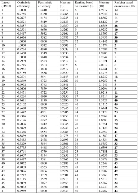
burden of measure (3), and a rounding error. It is clear that measure (10) is more efficient, and can save a lot of calculations compared with measure (3). A similar problem exists in Table 4. The ranking based on measures (3) and (10) has changed the results of 26 AMTs. That is, more than 55% of AMTs are ranked wrongly. We have shown them in bold font. This is the biggest advantage of measure (10) over measure (3) for AMT selection and justification.
Table 2: Evaluation of the 12 industrial robots by DEA with double frontiers
Robot Optimistic efficiency
Pessimistic efficiency
Measure (3)
Ranking based on measure (3)
Measure (10)
Ranking based on measure (10)
1 1.0000 1.0146 0.5670 7 1.4246 7
2 1.0000 1.0000 0.5631 8 1.4142 8
3 0.9824 1.1193 0.5898 5 1.4892 5
4 1.0000 1.1921 0.6144 2 1.5560 2
5 1.0000 1.2227 0.6226 1 1.5796 1
6 1.0000 1.1515 0.6036 4 1.5251 4
7 1.0000 1.1587 0.6055 3 1.5306 3
8 0.9614 1.0748 0.5717 6 1.4421 6
9 1.0000 1.0000 0.5631 8 1.4142 8
10 0.9536 1.0000 0.5494 11 1.3818 11
11 0.9831 1.0000 0.5581 10 1.4023 10
12 0.8012 1.0000 0.5043 12 1.2814 12
Table 3: Evaluation 21 the CNC lathes by DEA with double frontiers
CNC lathe
Optimistic efficiency
Pessimistic efficiency
Measure (3)
Ranking based on measure (3)
Measure (10)
Ranking based on measure (10)
1 1.0000 1.2133 0.4561 6 1.5723 6
2 0.8351 1.1183 0.3997 18 1.3957 18
3 0.8746 1.3936 0.4583 5 1.6453 5
4 1.0000 1.8121 0.5630 1 2.0697 1
5 0.9345 1.0833 0.4172 14 1.4307 15
6 0.8177 1.0000 0.3744 20 1.2917 20
7 0.5401 1.0000 0.3079 21 1.1365 21
8 1.0000 1.0715 0.4308 12 1.4657 13
9 1.0000 1.1634 0.4472 7 1.5341 7
10 0.8457 1.2346 0.4230 13 1.4965 11
11 0.8193 1.1960 0.4097 16 1.4497 14
12 1.0000 1.3867 0.4871 3 1.7096 3
13 0.8889 1.2326 0.4329 10 1.5197 8
14 1.0000 1.3929 0.4882 2 1.7147 2
15 1.0000 1.0785 0.4321 11 1.4708 12
16 0.9625 1.1476 0.4354 9 1.4978 9
17 0.9182 1.0691 0.4108 15 1.4092 16
18 0.8983 1.0581 0.4040 17 1.3880 19
19 0.9144 1.4144 0.4715 4 1.6842 4
20 0.7576 1.1879 0.3935 19 1.4089 17
Table 4: Evaluation of the 47 alternative machine component grouping solutions by DEA with double frontiers
Layout (DMU)
Optimistic efficiency
Pessimistic efficiency
Measure (3)
Ranking based on measure (3)
Measure (10)
Ranking based on measure (10)
1 1.0000 1.6410 0.3312 8 1.9217 12
2 0.9765 1.6350 0.3266 11 1.9044 13
3 0.9697 1.6184 0.3238 14 1.8867 14
4 0.9521 1.5419 0.3133 19 1.8122 19
5 0.7887 1.4328 0.2750 29 1.6355 28
6 0.9591 1.6670 0.3269 9 1.9232 10
7 0.9417 1.5932 0.3166 15 1.8507 17
8 0.8656 1.3382 0.2785 27 1.5937 30
9 1.0000 1.0000 0.2674 32 1.4142 38
10 1.0000 1.9342 0.3603 2 2.1774 2
11 0.9224 1.4970 0.3038 21 1.7584 21
12 0.9450 1.7519 0.3330 7 1.9905 7
13 1.0000 1.9648 0.3634 1 2.2047 1
14 0.9939 1.8523 0.3512 4 2.1021 4
15 0.9715 1.7503 0.3373 6 2.0019 6
16 0.7961 1.1808 0.2512 37 1.4241 37
17 0.8159 1.2558 0.2620 34 1.4976 34
18 0.9501 1.5561 0.3143 18 1.8232 18
19 0.9549 1.6723 0.3267 10 1.9257 9
20 0.9972 1.8763 0.3541 3 2.1249 3
21 0.9606 1.7879 0.3392 5 2.0296 5
22 0.9471 1.6722 0.3254 12 1.9218 11
23 0.9264 1.6030 0.3150 17 1.8514 16
24 0.7611 1.1179 0.2390 39 1.3523 40
25 0.6102 1.0000 0.2020 46 1.1715 46
26 0.8670 1.3969 0.2846 26 1.6441 26
27 0.8442 1.4961 0.2906 24 1.7178 23
28 0.9316 1.6973 0.3253 13 1.9362 8
29 0.9176 1.6272 0.3160 16 1.8680 15
30 0.9006 1.5412 0.3046 20 1.7851 20
31 0.8829 1.4675 0.2943 22 1.7126 24
32 0.7346 1.0554 0.2284 42 1.2859 41
33 0.5839 1.0000 0.1975 47 1.1580 47
34 0.7453 1.2478 0.2493 38 1.4534 36
35 0.7229 1.3544 0.2561 36 1.5352 33
36 0.7755 1.4448 0.2740 30 1.6398 27
37 0.8761 1.4779 0.2941 23 1.7181 22
38 0.8607 1.4144 0.2853 25 1.6557 25
39 0.8417 1.3581 0.2765 28 1.5978 29
40 0.7072 1.0000 0.2183 45 1.2248 45
41 0.7003 1.0565 0.2227 43 1.2675 44
42 0.6826 1.0836 0.2224 44 1.2807 42
43 0.6717 1.1789 0.2301 41 1.3568 39
44 0.8115 1.3569 0.2713 31 1.5810 31
45 0.8039 1.3097 0.2653 33 1.5367 32
46 0.8032 1.2585 0.2601 35 1.4930 35
4. Conclusion
In this note, we point to computational errors in the paper by Wang and Chin (2009). We showed that their proposed measure for ranking AMTs can be problematic. To overcome these problems, we proposed another measure for ranking AMTs. Numerical examples show that the proposed measure can rank all AMTs correctly. The proposed measure is expected to play an important role in AMT selection and justification and to have more applications in the future.
References
1. Azizi, H. & Wang, Y.-M. (2013). Improved DEA models for measuring interval efficiencies of decision-making units. Measurement, 46(3), 1325-1332.
2. Charnes, A., Cooper, W.W. & Rhodes, E. (1978). Measuring the efficiency of decision making units. European Journal of Operational Research, 2(6), 429-444.
3. Liu, F.-H.F. & Chen, C.L. (2009). The worst-practice DEA model with slack-based measurement. Computers & Industrial Engineering, 57(2), 496-505.
4. Wang, Y.-M. & Chin, K.-S. (2009). A new approach for the selection of advanced manufacturing technologies: DEA with double frontiers. International Journal of Production Research, 47(23), 6663-6679.