Open Access
Research
Method of predicting Splice Sites based on signal interactions
Alexander Churbanov*
1, Igor B Rogozin
2, Jitender S Deogun
3and
Hesham Ali
1Address: 1Department of Computer Science, College of Information Science and Technology, University of Nebraska at Omaha, Omaha,
NE68182-0116, USA, 2NCBI/NLM/NIH, Bldg.38-A, room 5N505A, 8600 Rockville Pike, Bethesda, MD 20894, USA and 3Department of
Computer Science and Engineering, University of Nebraska-Lincoln, Lincoln, NE 68588-0115, USA
Email: Alexander Churbanov* - [email protected]; Igor B Rogozin - [email protected]; Jitender S Deogun - [email protected]; Hesham Ali - [email protected]
* Corresponding author
Abstract
Background: Predicting and proper ranking of canonical splice sites (SSs) is a challenging problem in bioinformatics and machine learning communities. Any progress in SSs recognition will lead to better understanding of splicing mechanism. We introduce several new approaches of combining a priori knowledge for improved SS detection. First, we design our new Bayesian SS sensor based on oligonucleotide counting. To further enhance prediction quality, we applied our new de novo motif detection tool MHMMotif to intronic ends and exons. We combine elements found with sensor information using Naive Bayesian Network, as implemented in our new tool SpliceScan.
Results: According to our tests, the Bayesian sensor outperforms the contemporary Maximum Entropy sensor for 5' SS detection. We report a number of putative Exonic (ESE) and Intronic (ISE) Splicing Enhancers found by MHMMotif tool. T-test statistics on mouse/rat intronic alignments indicates, that detected elements are on average more conserved as compared to other oligos, which supports our assumption of their functional importance. The tool has been shown to outperform the SpliceView, GeneSplicer, NNSplice, Genio and NetUTR tools for the test set of human genes. SpliceScan outperforms all contemporary ab initio gene structural prediction tools on the set of 5' UTR gene fragments.
Conclusion: Designed methods have many attractive properties, compared to existing approaches. Bayesian sensor, MHMMotif program and SpliceScan tools are freely available on our web site.
Reviewers: This article was reviewed by Manyuan Long, Arcady Mushegian and Mikhail Gelfand.
Open peer review
Reviewed by Manyuan Long, Arcady Mushegian and Mikhail Gelfand. For the full reviews, please go to the Reviewers' comments section.
Background
Precise removal of introns from pre-messenger RNAs (pre-mRNAs) by splicing is a critical step in expression of most metazoan genes. The process requires accurate recogni-tion and pairing of 5' and 3' SSs by the splicing machinery. Inappropriate splicing of a gene may result in the transla-Published: 03 April 2006
Biology Direct 2006, 1:10 doi:10.1186/1745-6150-1-10
Received: 03 March 2006 Accepted: 03 April 2006
This article is available from: http://www.biology-direct.com/content/1/1/10
© 2006 Churbanov et al; licensee BioMed Central Ltd.
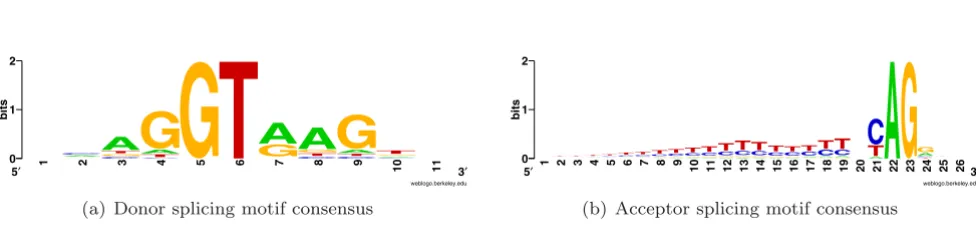
tion of a nonfunctional protein. SS motifs are necessary, but not sufficient, for the exact recognition of the exons. Frequently degenerate donor, acceptor and branch point motifs provide insufficient information for exact SS detec-tion [1]. Figure 1 shows SS consensus signals for both 5' and 3' exonic ends. The human transcribed regions have plenty of motifs of unknown functionality with structure very similar to the SS consensus signals (GT or AG dinu-cleotide surrounded by proper context). These sites are called splice-like signals and they outnumber the real sites by several orders of magnitude.
Correct prediction of SSs appears to be the key ingredient in successful ab initio gene annotation, since dynamic pro-gramming procedures must see all the exon/intron boundaries in order to find the optimal solution [2]. The most sensitive sensor design predicting the least amount of false positives is preferable. Another good feature of a SS sensor is the ability to rank predicted SSs, i.e. to assign a certain score characterizing the importance or strength of a putative site of splicing.
Numerous approaches have been taken towards effective detection of SSs. In our experiments, the highest perform-ance for complete gene structural prediction has been achieved with GenScan [3] and HMMgene [4] tools. Both tools use three-periodicity in coding exons. Codonic com-position of coding exons has particular probabilistic prop-erties that allow gene finders to synchronize their prediction engines with gene structure and efficiently stitch exons in frame-consistent fashion [2].
However, all tools relying on three-periodic coding com-ponents in their prediction algorithm suffer substantial performance loss if confronted with noncoding exons. On the other hand, the biological splicing process seems to be indifferent to exonic coding potential [5,6]. To alleviate the problem, gene structural prediction tools use
informa-tion sources directly related to the biological process of splicing [7]. One of the promising mechanisms of SS def-inition is signal interaction, i.e. putative SSs and various ESEs, ISEs in addition to Exonic (ESS) and Intronic (ISS) Splicing Silencers [see Subsection Splicing signals].
In this paper we introduce our new gene structural anno-tation tool SpliceScan. Our tool is based on the Naive Bayesian network that linearly combines the number of splicing-related components to improve SS prediction. Before we describe our tool, we discuss our approach to SS sensor design [see Subsection Splice Sites sensor]. We dis-cuss the MHMMotif tool we use to detect putative splicing enhancers [see Subsection De novo motifs detection].
Splicing signals
Specificity in the splicing process derives partly from sequences other than SS signals, including Exonic Splicing Enhancer (ESE) and Exonic Splicing Silencer (ESS) signals [8,9]. ESE signals are required for a constitutive exon def-inition and for an efficient splicing of weak alternatively spliced exons [10] (while ESS signals suppress the removal of adjacent introns [9,11]), which may lead to exon skipping. There are 10 serine/arginine-rich (SR) Splicing Enhancer proteins known today (SRp20, SC35, SRp46, SRp54, SRp30c, SF2/ASF, SRp40, SRp55, SRp75, 9G8 [12]) and approximately 20 hnRNP Splicing Silenc-ing factors [13], among them the most studied hnRNP A1 complex [11]. Tra2β is reported to be the SR splicing reg-ulator [12]. All the SR proteins have two structural motifs: the RNA Recognition Motif (RRM) binding to certain motifs in RNA; and the arginine/serine-rich (RS) domain responsible for Protein-Protein interactions within splic-ing complex [12].
Together with inefficient SS signals, the appropriate bal-ance of ESE and ESS elements somehow allows fine tun-ing of the splictun-ing mechanism [9]. Both 5' U1 snRNP and Consensus motifs for donor and acceptor SSs
Figure 1
Consensus motifs for donor and acceptor SSs. Y-axis indicates the strength of base composition bias based on information content.
weblogo.berkeley.edu
0 1 2
bits
5′ 1 2
GA
C
3
C
GAT
4
CT
A
G
5
G
T
6 CG7A
8
C
T
G
A
9
CTA
G
10
CA
GT
11 3′
(a) Donor splicing motif consensus
weblogo.berkeley.edu
0 1 2
bits
5′ 1 2
T
3
C
T
4
C
T
5
C
T
6
A C
T
7
G
A C
T
8
A
G
C
T
9
A
G
CT
10
A
G
C
T
11
A
G
C
T
12
A
G
CT
13
A
G C
T
14
A
G CT
15
A
G
C T
16
A
G
CT
17
G
A C T
18
G
A
CT
19
G
A
CT
20 21
A
T
C
22
A
G
23 24T
C
A
G
25
T
26 3′
3' U2AF65·U2AF35 were shown to interact with ESEs [12].
Cross-intron bridging may happen through hnRNP com-plexes [14]. Experiments show that the 3' end definition is not affected by intron bridging, but is defined solely by the strength of the acceptor site polypyrimidine tract and the position of splicing enhancers and silencers [10,15].
The silencing process is still poorly understood [16]. However, there are several models explaining the observed antagonism between hnRNP complexes and SR proteins [17]. For example, hnRNP A1 binds to the ESS and hinders binding of SR proteins to a weak ESE located just downstream of ESS [9]. Several rules have been iden-tified for interaction of ESE/ESS factors with spliceosomal assembly:
• ESE and ESS elements are frequently located in down-stream exons [18];
• The precise mechanism by which hnRNP A1 binds the ESS in the upstream exon and represses splicing of the upstream intron remains unknown, although the 3' site is a likely target for repression [9] as shown in Figure 2(c);
• Most splicing enhancers are located within 100 nucleo-tides of the 3' SS and are not active further away [15];
• Each enhancer complex assembles independently for 3' and 5' sites, and there is a minor interaction across an intron [19], as shown in Figure 2(a);
• Based on current views of exon definition, each exon should be recognized by the splicing machinery as an independent unit [3,19], as shown in Figure 2(b);
• Analysis of the experimental data revealed that the splic-ing efficiency is directly proportional to the calculated probability of a direct interaction between the enhancer complex and the 3' SS:
- Strong natural enhancers function at a greater distance from the intron than weak natural enhancers do [18];
- The closer an ESE is to a SS, the more efficient it is [15];
- Multiple enhancer sites increase the probability of splic-ing activation [15];
- Strong ESS sites may suppress an effect from ESE(s) located upstream [9].
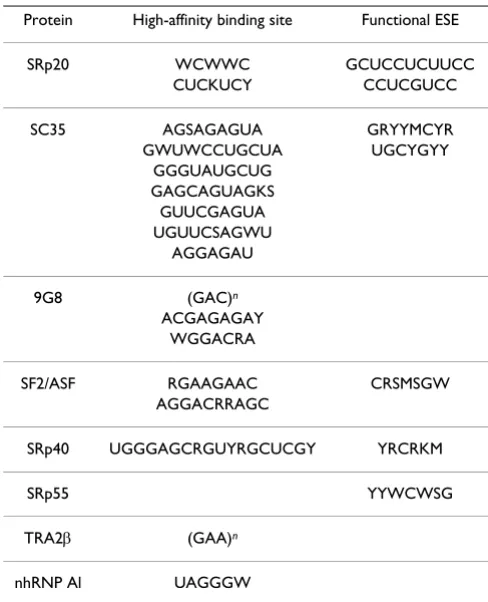
To identify known ESE/ESS motifs, we used RRM binding motifs from [20] as shown in Table 1. PolyA signals, that could also be employed by splicing machinery, were detected by oligos reported in [21].
Results and discussion
Bayesian sensor performanceWe use the Receiver Operating Characteristic (ROC) to compare performance of different sensors. A ROC curve is a graphical representation of the tradeoff between the false negative and false positive rates for every possible cutoff. By tradition, the plot shows the false positive rate (1 - Specificity) on the x axis and the false negative rate (Sensitivity) on the y axis.
Sensitivity (Sn) and Specificity (Sp) were calculated according to the formulas
Here TE is the number of accurately predicted exon boundaries, AE is the number of annotated exon bounda-ries in the test set and PE is the number of predicted exon boundaries.
The accuracy of a test (i.e. the ability of the test to correctly classify cases with a certain condition and cases without
Sn TE AE
=
( )
1Sp TE PE
=
( )
2Models of exon definition and ESS-ESE interaction
Figure 2
Models of exon definition and ESS-ESE interaction.
SR protein
ESE
SR protein
ESE GU AG Exon 2 Exon 1
U1 snRNP
A Py 70K
U2AF65
U2AF35
(a) SSs recognition
SR protein
AG GU
U1 snRNP
ESE Exon A Py
U2AF65
U2AF35 70K
(b) Exon definition model
SR protein
ESE
AG Exon ESS hn RNP
A Py
U2AF65
U2AF35
the condition) is measured by the area under the ROC curve. An area of 1 represents a perfect test. The closer the curve follows the left-hand and top borders of the ROC space, the more accurate the test; i.e. the true positive rate is high and the false positive rate is low. Statistically, more area under the curve means that it is identifying more true positives while minimizing the number of false positives.
To evaluate Bayesian sensor performance we compiled three test sets:
1. 250 first multiexonic all-canonical SS genes picked from the top of our GIGOgene annotation. This test set includes 2,482 donor and 347,402 donor-like signals in addition to 2,482 acceptor and 465,000 acceptor-like sig-nals.
2. 1,072 human 5' UTR gene-annotated fragments, including the first 50 nt from the CDS region. We picked only GIGOgene annotations containing at least one intron with all canonical SSs. Our 5' UTR test set includes 1,869 donor and 734,744 donor-like signals in addition to 1,846 acceptor and 925,464 acceptor-like signals.
3. 183 rat multiexonic all-canonical SS genes we were able to annotate with GIGOgene. This test set includes 1,405
donor and 240,539 donor-like signals in addition to 1,405 acceptor and 295,640 acceptor-like signals. The test set is specifically included to evaluate cross-specie sensor performance.
For experimental purposes on human test sets we removed cross-correlating gene-annotated fragments from the learning set. In experiments with human test sets we BLAST-aligned the test set to the learning set and removed all homologous fragments, both human and mouse, with BLASTN hit expected value less than 10-10
and bitscore more than 75 bits. The experimental sensor performance study is shown in Figure 4. ROC curve irreg-ularities could be attributed to multimodal score distribu-tion of splice and splice-like signal, as could be seen in Figure 3. We did not removed cross-correlation between the learning set and the test set of 183 rat genes.
Our Bayesian 5' SS sensor outperforms the recently intro-duced Maximum Entropy SS sensor [22] and MDD sensor used in GenScan tool [3] as could be seen in Figures 4(a), 4(c) and 4(e). Performance of the Bayesian 3' SS sensor is similar to that of the Maximum Entropy SS sensor [22].
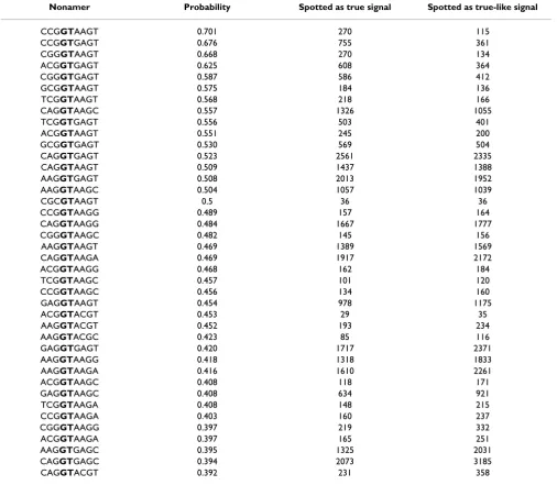
The 5' SS oligonucleotides tend to cluster, only 3,084 non-amers got non-zero probability entries in the sensor table, with the highest 40 ranked motifs shown in Table 2. Among 2,482 true 5' SSs tested in the test set of 250 human genes, 13 nonamers had zero entries in the table which stands for oligonucleotide miss rate of 0.52%. On the other hand, acceptor SSs demonstrates great variabil-ity and requires substantially larger learning sets [see Sub-section Learning set size study].
Bayesian 3' SS sensor design seems to favor correla-tion between the learning set and test sequences; cross-correlation removal worsened sensor ROC characteristics [see Subsection Learning and test sets cross-correlation degree study]. In reality, sensor performance should be as good or better than reported because we used an extensive set of genes in human and mouse genomes for learning, cover-ing most gene families. Chances are high that a sequence in question substantially cross-correlates with the learning set we use. Test example with 183 rat genes confirms our expectations, as could be seen in Figure 4(f), where ROC of the Bayesian sensor prevails over all other sensor designs.
Learning and test sets cross-correlation degree study
We study Bayesian sensor performance depending on the degree of cross-correlation between the learning and test sets. Test performance appears to be the best for experi-ments with intersecting test and learning sets, denoted as "Bayesian" in Figure 5. Removal of test set sequences from the learning set corresponds to curves denoted as "Baye-Table 1: Nucleotide symbols used: M → (A/C), R → (A/G), W →
(A/U), Y → (C/U), S → (C/G), K → (G/U). (Table credit [20])
Protein High-affinity binding site Functional ESE
SRp20 WCWWC GCUCCUCUUCC CUCKUCY CCUCGUCC
SC35 AGSAGAGUA GRYYMCYR GWUWCCUGCUA UGCYGYY
GGGUAUGCUG GAGCAGUAGKS GUUCGAGUA UGUUCSAGWU
AGGAGAU
9G8 (GAC)n ACGAGAGAY
WGGACRA
SF2/ASF RGAAGAAC CRSMSGW AGGACRRAGC
SRp40 UGGGAGCRGUYRGCUCGY YRCRKM
SRp55 YYWCWSG
TRA2β (GAA)n
sian (validation)" and further elimination of cross-correlating sequences [see Subsection Bayesian sensor per-formance] corresponds to "Bayesian (no cross-correla-tion)" curves in Figure 5. Cross-correlation removal has a dramatic effect on the performance of the 3' SS sensor as shown in Figure 5(b). On the other hand, cross-correla-tion has practically no effect on the performance of the 5' SS sensor as shown in Figure 5(a).
Learning set size study
Our experiments with learning set size indicate, that 5' SS performance tolerates substantial decimation of the learn-ing set without apparent quality loss, as shown in Figure 6(a). Decreased size of learning set causes substantial per-formance loss for 3' SS sensor, as shown in Figure 6(b).
The learning set we collected [see Subsection Splice Sites sensor] is not sufficiently vast for 3' SS sensor to avoid per-formance loss in case of removed cross-correlation. Ideal 3' SS ROC curve should be similar to the "Bayesian" as shown in Figure 5(b).
Detection of ISE signals
ISE motifs are essential components for understanding splicing events. In order to predict ISE motifs located in vicinity of 3' and 5' SS, we compiled two sample sets of 2,000 pre-donor and post-acceptor 150 nt fragments known to be real with a high degree of confidence. For fragment extraction we parsed results of GIGOgene [23] spliced alignment of human RefSeq against the phase III
human DNA database from NCBI, picking only canonical SSs from predicted multiexonic structures.
We applied MHHMotif to these sample sets of sequences, and recovered motifs shown in Figure 7, where represent-ative motifs were obtained from HMM components in "generative mode" [see Additional file 1].
Intronic conservation study
We adopt conservation criteria to evaluate significance of the putative ISE elements found [see Additional file 1]. We subdivided set of all possible 8-mer oligonucleotides in two subsets: hypothesis subset, i.e. all detected putative ISE elements, and null-hypothesis subset – the rest of the possi-ble oligos. To study evolutionary conservation we took 3,005 mouse-rat intronic alignments. In our conservation study we considered only first 100 nt and last 100 nt of each alignment, excluding very first 5 nt and very last 5 nt for they playing role in SS highly conserved consensus sig-nals.
We used sliding window of size 8 nucleotides to detect positions matching the set of detected putative ISEs. Ratios of conserved nucleotide positions vs. non-con-served nucleotide positions were calculated for our hypo-thesis set and null-hypohypo-thesis set elements. We removed test pairs where either ISEs were not detected or non of the nucleotides within putative ISEs changed. Alignments too short to extract statistics regions were also removed. Bayesian sensor histograms produced for 5' SS and 3' SS signals on the test set of 250 human genes
Figure 3
Bayesian sensor histograms produced for 5' SS and 3' SS signals on the test set of 250 human genes.
ROC diagrams for Donor and Acceptor signals
Figure 4
ROC diagrams for Donor and Acceptor signals.
40 50 60 70 80 90 100 0
10 20 30 40 50 60 70 80 90
Donor ROC curve
False positives
Sensitivity
WMM MM MDD Maximum entropy SpliceView
Bayesian (no cross−correlation)
(a) Sensors ROC diagram for 5SS (test set of 250 human genes)
55 60 65 70 75 80 85 90 95 100 0
10 20 30 40 50 60 70 80 90
Acceptor ROC curve
False positives
Sensitivity
Maximum Entropy MM WMM SpliceView
Bayesian (no cross−correlation)
(b) Sensors ROC diagram for 3SS (test set of 250 human genes)
60 65 70 75 80 85 90 95 100 0
10 20 30 40 50 60 70 80 90
Donor ROC curve
False positives
Sensitivity
WMM MM MDD Maximum entropy SpliceView
Bayesian (no cross−correlation)
(c) Sensors ROC diagram for 5 SS (test set of 5 UTR fragments)
80 85 90 95 100 0
10 20 30 40 50 60 70 80 90
Acceptor ROC curve
False positives
Sensitivity
Maximum Entropy MM WMM SpliceView
Bayesian (no cross−correlation)
(d) Sensors ROC diagram for 3 SS (test set of 5 UTR fragments)
40 50 60 70 80 90 100 0
10 20 30 40 50 60 70 80 90 100
Donor ROC curve
False positives
Sensitivity
WMM MM MDD Maximum entropy SpliceView Bayesian split−sample
(e) 5SS (test set of 183 rat genes)
55 60 65 70 75 80 85 90 95 100 0
10 20 30 40 50 60 70 80 90
Acceptor ROC curve
False positives
Sensitivity
Maximum Entropy MM WMM SpliceView Bayesian split−sample
The following probabilities associated with a two-tailed Student's paired t-test were found as shown in Table 3. Detected putative ISE elements are on average more con-served than other oligos. Statistically significant higher evolutionary conservation suggests the biological impor-tance of a significant fraction of these elements in the splicing process.
Detecting ESE signals
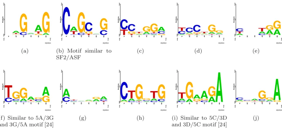
To detect putative ESE signals we applied the MHMMotif tool to the set of 2,000 distinct exons as we parsed the human genome annotation of our GIGOgene tool. In our experiments, motifs in Figures 8(a), 8(b), 8(c), 8(f), and
8(h) converged in two families with similar ESE signal sig-nature but different convolution patterns supporting either 5' or 3' exonic ends. We present putative motifs [see Additional file 1]. Our set of putative ESE signals substan-tially overlaps with ESEs suggested by Burge and co-work-ers [24]. Among 202 detected putative ESE elements, 42 are present in this previously reported set of 238 ESEs, which exceeds randomly expected overlap by 3.5 times. Strong evolutionary conservation was found for these ESE signals located near splicing signals [25].
Table 2: Probabilities of being true SS for first 40 statistically most highly ranked putative 5' SS. Probabilities are calculated based on number of times we spot certain nonamer acting as SS as opposed to splice-like signal in our learning set [see Subsection Splice Sites sensor]
Nonamer Probability Spotted as true signal Spotted as true-like signal
CCGGTAAGT 0.701 270 115
CCGGTGAGT 0.676 755 361
CGGGTAAGT 0.668 270 134
ACGGTGAGT 0.625 608 364
CGGGTGAGT 0.587 586 412
GCGGTAAGT 0.575 184 136
TCGGTAAGT 0.568 218 166
CAGGTAAGC 0.557 1326 1055
TCGGTGAGT 0.556 503 401
ACGGTAAGT 0.551 245 200
GCGGTGAGT 0.530 569 504
CAGGTGAGT 0.523 2561 2335 CAGGTAAGT 0.509 1437 1388 AAGGTGAGT 0.508 2013 1952 AAGGTAAGC 0.504 1057 1039
CGCGTAAGT 0.5 36 36
CCGGTAAGG 0.489 157 164
CAGGTAAGG 0.484 1667 1777
CGGGTAAGC 0.482 145 156
AAGGTAAGT 0.469 1389 1569 CAGGTAAGA 0.469 1917 2172
ACGGTAAGG 0.468 162 184
TCGGTAAGC 0.457 101 120
CCGGTAAGC 0.456 134 160
GAGGTAAGT 0.454 978 1175
ACGGTACGT 0.453 29 35
AAGGTACGT 0.452 193 234
AAGGTACGC 0.423 85 116
GAGGTGAGT 0.420 1717 2371 AAGGTAAGG 0.418 1318 1833 AAGGTAAGA 0.416 1610 2261
ACGGTAAGC 0.408 118 171
GAGGTAAGC 0.408 634 921
TCGGTAAGA 0.408 148 215
CCGGTAAGA 0.403 160 237
CGGGTAAGG 0.397 219 332
ACGGTAAGA 0.397 165 251
AAGGTGAGC 0.395 1325 2031 CAGGTGAGC 0.394 2073 3185
SpliceScan performance
We use test sets [see Subsection Bayesian sensor perform-ance] for the SpliceScan performance estimates. We chose the second test set of non-coding 5' UTRs because it was suggested that at least some introns in 5' UTRs may atten-uate translation at the initiation stage [26,27]. Thus, a reli-able prediction of introns and strength of splicing signals in 5' UTRs is essential for 5' UTR studies.
Performance of SpliceScan appears to be the best for short non-coding 5' UTR gene fragments test set, as presented in Figures 9(e) and 9(f). For the test set of 250 human genes and 183 rat genes our tool predicts SSs better than SpliceView [5], GeneSplicer [28], NNSplice [29], Genio [30] and NetUTR [6].
Study of cross-correlation performance dependency
Figure 5
Study of cross-correlation performance dependency.
50 60 70 80 90 100
0 10 20 30 40 50 60 70 80 90
Donor ROC curve
False positives
Sensitivity
Bayesian (no cross−correlation) Bayesian (cross−validation) Bayesian
Maximum Entropy
(a) 5SS (test set of 250 human genes)
55 60 65 70 75 80 85 90 95 100 0
10 20 30 40 50 60 70 80 90
Acceptor ROC curve
False positives
Sensitivity
Bayesian (no cross−correlation) Bayesian (cross−validation) Bayesian
Maximum Entropy
(b) 3SS (test set of 250 human genes)
Study of sensor performance based on learning set size
Figure 6
Study of sensor performance based on learning set size.
50 55 60 65 70 75 80 85 90 95 100 10
20 30 40 50 60 70 80 90 100
Donor ROC curve
False positives
Sensitivity
Full learning set Quarter of learning set Sixteenth of learning set
(a) 5 SS (test set of 250 human genes)
60 65 70 75 80 85 90 95 100 10
20 30 40 50 60 70 80 90 100
Acceptor ROC curve
False positives
Sensitivity
Full learning set Half of learning set Quarter of learning set
Conclusion
By trading complexity of sensor design for the size of learning set we were able to substantially improve predic-tion of the SSs. Bayesian 5' SS sensor demonstrated supe-rior performance, as compared to existing approaches, in all conducted experiments. Neither removal of cross-cor-relation between the learning and test set, nor fourfold decrease of learning set size were able to compromise the sensor fidelity. Opposite observation were made with 3' SS sensor, where performance is affected both by degree of cross-correlation between learning and test set and the size of the learning set. Bayesian 3' SS sensor demonstrates comparable performance with the Maximum Entropy sensor, when cross-correlation is removed between the learning and test set. The sensor performance improves substantially if we do not specifically remove cross-corre-lation, as in case of 183 rat genes test set or experiments with the degree of cross-correlation. We believe that per-formance of our sensor could be generalized to a broad variety of tetrapoda organisms; genes encoding splicing RNP complexes are among the most conserved known genes [31].
Using MHMMotif tool we were able to discover motif families for ESE/ISE elements. Small fraction of our detected putative ESE elements correspond to previously reported ESE motifs [24], other elements could be consid-ered as novel. Statistically significant average conservation ratio for putative ISE elements, as compared to other motifs, supports their functional importance in human genome.
Our predicted ISE and ESE elements have substantial impact on splicing, as we were able to improve SS predic-tion using these elements. Based on linear model of splic-ing factors interaction, SpliceScan has been able to outperform SpliceView [5], GeneSplicer [28], NNSplice [29], Genio [30] and NetUTR [6] tools in all the test cate-gories.
SpliceScan did not to perform better than GenScan [3], HMMgene [4], NetGene2 [32,33], MZEF [34], Geneid [35,36] and ExonScan [7] on the test set 250 human genes and 183 rat genes. The reason is that SpliceScan does not rely on three periodicity property to discover the coding exons. ExonScan, which uses exon definition model com-bined with ESS/ESE elements for better prediction quality, ISE motifs found in vicinity of 3' SS (Figures 7(a)-7(g)) and 5' SS (Figures 7(h)-7(m))
Figure 7
ISE motifs found in vicinity of 3' SS (Figures 7(a)-7(g)) and 5' SS (Figures 7(h)-7(m)).
ISE signals related to Acceptor
weblogo.berkeley.edu
0 1 2
bits
5′ 1
A G C T 2 A G C T 3 G C
T
4 G CT 5 A G CT 6 G A C T 7C
T
8 CT
3′ (a) weblogo.berkeley.edu 0 1 2 bits5′ 1
T
G
2 CG
3 A T CG
4 T G C 5 A GT 6 A CG
7 TG
G
8 3′ (b) weblogo.berkeley.edu 0 1 2 bits5′ 1
T
C
2 AC
3 GTC
4 A G CT 5 CTG
6 G AC
7 A T GC
8 A T GC
3′ (c) weblogo.berkeley.edu 0 1 2 bits5′ 1
C A
T
2 A G CT
3 G A CT
4 A G CT 5 G A CT 6 G A CT
7 A CT
8 CT
3′ (d) weblogo.berkeley.edu 0 1 2 bits5′ 1
A C
T
2 AT
3 A GT
4 G A CT
5 G CT A 6 G T CA
7 G TA
8 G TA
3′ (e) weblogo.berkeley.edu 0 1 2 bits5′ 1 G T A 2 C T A 3 CT A 4 G T C
A
5CT
A
6 C G
A
7 G TA
8 G CA
3′ (f) weblogo.berkeley.edu 0 1 2 bits5′T1
C
2 G T C 3 GT C 4 A G CT
5 GT C 6 GT
C
7 T GC
C
8T
3′
(g)
ISE signals related to Donor
weblogo.berkeley.edu
0 1 2
bits
5′
A
1T
2 AT
3 GAT
4 C G A T 5 G TA
6 G AT
7T
A
8A
T
3′ (h) weblogo.berkeley.edu 0 1 2 bits5′ 1 G
C
2 TC
3 A GC
4 G C A 5 T C A G 6 A T C G 7 A T G C 8 A GC
3′ (i) weblogo.berkeley.edu 0 1 2 bits5′ 1 GA
T
2 GA CT 3 G CA T 4 A C G T 5 G A C T 6 C T A 7 CA T 8
A
T
3′ (j) weblogo.berkeley.edu 0 1 2 bits5′ 1
T C
G
2 A CTG
3 T GC
4 T 5 C T G 6 T CG
7 T AG
8G
3′(k) weblogo.berkeley.edu 0 1 2 bits
5′ 1
C
G
2 CTG
3 T A CG
4 T G C 5 G A T 6 C A TG
7 TG
8 AG
3′(l) weblogo.berkeley.edu 0 1 2 bits
5′
C
1 2is another tool implemented as splicing simulator with objectives similar to SpliceScan. It has the same "average" ROC profile for not using exonic coding potential statis-tics. Exon definition model of ExonScan seems to work better for internal boundaries prediction, but suffers in case of predicting boundaries of incomplete exons, first and last exons, as all the other tools do.
In our experiments on the human test sets we removed cross-correlation from the learning set, that made per-formance of our tool worse as it would normally be. Since we do not have control over the learning sets of the com-peting tools, performance of these tools is likely to be pos-itively affected by overlaps between their learning sets and our test sets. The test set of 183 rat genes exemplifies the performance issues with the existing tools that were trained on the human learning sets; they usually perform worse when confronted with new sequences. ExonScan does not seem to lose prediction quality when confronted with sequences from other closely related organisms.
SpliceScan performs best on the set 5' UTR fragments because of the SS definition model we use, i.e. we combine all available information for a certain SS without manda-tory requirement of large contexts or having other corre-sponding exonic boundary.
Bayesian sensor, MHMMotif program and SpliceScan tools are freely available on our web site [37].
Methods
Splice Sites sensorSSs are known to contain complex interdependencies between nonadjacent positions that could be attributed to evolutionary pressure from very complex biological splic-ing machinery. Recovery of these interdependencies is dif-ficult problem in machine learning, but may lead to better understanding of the splicing process and improved sen-sor design.
Numerous approaches have been taken towards effective detection of SS [38-50]. The earliest SS sensors were the Table 3: T-test probabilities for putative ISE elements found
Putative ISE elements Test area Number of alignments Probability
Donor-related ISEs Post-donor region 2,544 7.22 × 10-82
Donor-related ISEs Pre-acceptor region 2,586 1.86 × 10-106
Acceptor-related ISEs Pre-acceptor region 2,487 8.39 × 10-95
Acceptor-related ISEs Post-donor region 2,235 6.39 × 10-59
ESE motifs repetitively detected in our MHHMotif runs
Figure 8
ESE motifs repetitively detected in our MHHMotif runs.
weblogo.berkeley.edu
0 1 2
bits
5′ 1 2
C GT A 3 C
G
4 T G C A 5 GTA
6 AG
3′ (a) weblogo.berkeley.edu 0 1 2 bits5′ 1
T
C
2 CT A 3 CG
4 T GC
5 T CA 6C
G
3′(b) Motif similar to SF2/ASF weblogo.berkeley.edu 0 1 2 bits
5′ 1
T
C
2 T GC
3 A GT 4 T CAG
5 ACT
G
6 G CA 3′ (c) weblogo.berkeley.edu 0 1 2 bits
5′ 1 A CT 2 T G A C 3 A T G
C
4 C G A T 5 C T AG
6 T C A G 3′ (d) weblogo.berkeley.edu 0 1 2 bits5′ 1 A
T
C
2 3 4 C A T 5 T A G 6
A
G
3′ (e) weblogo.berkeley.edu 0 1 2 bits5′ 1
C
T
2 T A CG
3 CAG
4 C GT A 5 A C G 6G
A
3′(f) Similar to 5A/3G and 3G/5A motif [24]
weblogo.berkeley.edu
0 1 2
bits
5′ 1
T
C
A
2 A C T 3 T C A 4 T C G A 5 T CA G 6 T CA 3′ (g) weblogo.berkeley.edu 0 1 2 bits5′ 1 GA
C
2 CAT
3
CTA
G
4 A C G 5 CAT
6 A CG
3′ (h) weblogo.berkeley.edu 0 1 2 bits5′ 1 CA
T
2 AG
3 C T G A 4 C GA
5A
G
6A
3′(i) Similar to 5C/3D and 3D/5C motif [24]
weblogo.berkeley.edu
0 1 2
bits
5′ 1
ROC diagrams for Donor and Acceptor applications
Figure 9
ROC diagrams for Donor and Acceptor applications.
0 10 20 30 40 50 60 70 80 90 100 0
10 20 30 40 50 60 70 80 90 100
Donor ROC curve
False positives (%)
Sensitivity (%) ExonScan (ESEs+ESSs+GGG) GeneSplicer
Genio GenScan HMMgene 1.1 (sig. md.) NetGene2 NetUTR 1.0 NNSplice SpliceView SpliceScan (no CC) SpliceScan (no CC + enh.) MZEF
geneid
(a) 5SS (test set of 250 human genes)
0 10 20 30 40 50 60 70 80 90 100 0
10 20 30 40 50 60 70 80 90 100
Acceptor ROC curve
False positives (%)
Sensitivity (%) ExonScan (ESE,ESS,GGG) GeneSplicer Genio GenScan HMMgene 1.1 (sig. md.) NetGene2 NetUTR 1.0 NNSplice SpliceView SpliceScan (no CC) SpliceScan (no CC + enh.) MZEF
geneid
(b) 3SS (test set of 250 human genes)
0 10 20 30 40 50 60 70 80 90 100 0
10 20 30 40 50 60 70 80 90 100
Donor ROC curve
False positives (%)
Sensitivity (%)
ExonScan (ESEs+ESSs+GGG) GeneSplicer
Genio GenScan HMMgene 1.1 (sig. md.) NetGene2 NetUTR 1.0 NNSplice SpliceView SpliceScan (enh.) MZEF geneid
(c) 5SS (test set of 183 rat genes)
0 10 20 30 40 50 60 70 80 90 100 0
10 20 30 40 50 60 70 80 90 100
Acceptor ROC curve
False positives (%)
Sensitivity (%)
ExonScan (ESE,ESS,GGG) GeneSplicer Genio GenScan HMMgene 1.1 (sig. md.) NetGene2 NetUTR 1.0 NNSplice SpliceView SpliceScan (enh.) MZEF geneid
(d) 3SS (test set of 183 rat genes)
30 40 50 60 70 80 90 100 0
10 20 30 40 50 60 70 80 90
Donor ROC curve
False positives (%)
Sensitivity (%)
ExonScan (with ESEs,ESSs and intronic GGG) GeneSplicer
Genio GenScan
HMMgene 1.1 (in signal mode) NetGene2
NetUTR 1.0 NNSplice SpliceView
SpliceScan (no cross−correlation) SpliceScan (no cross−correlation plus Enhancers) MZEF
geneid
(e) 5SS (test set of 5 UTR fragments)
65 70 75 80 85 90 95 100 0
10 20 30 40 50 60 70 80 90
Acceptor ROC curve
False positives (%)
Sensitivity (%)
ExonScan (with ESEs,ESSs and intronic GGG) GeneSplicer
Genio GenScan
HMMgene 1.1 (in signal mode) NetGene2
NetUTR 1.0 NNSplice SpliceView
SpliceScan (no cross−correlation) SpliceScan (no cross−correlation plus enhancers) MZEF
geneid
Weight Matrix Model (WMM) [51], Weight Array Model (WAM) [52], and Windowed second-order WAM model (WWAM) [3]. The Maximal Dependence Decomposition (MDD) sensor mentioned in [3] outperformed previously known 5' SS sensors. It explores long-range dependencies in the donor 5' motif by iterative subdivision at each stage splitting on the most dependent position, suitably denned. Leaves of the resulting bifurcation tree appear to be simple WMM models. Another approach, published in parallel and implemented in the SpliceView program [5], explores the same idea of creating WMM motif families with a clustering algorithm, which leads to better per-formance compared to simple WMM and WAM.
Various sensors were built later or in parallel based on Bayesian Networks [53,54], Neural Networks [29,55] and Boltzmann machine with Bahadur expansion [56]. Also there was a recent study based on Support Vector Machine (SVM) [57]. None of these methods were shown to out-perform MDD for 5' SSs. A new Maximum Entropy sensor [22], Permuted Markov Models [58] and approach based on dependency graphs and their expanded Bayesian net-work [59] outperformed MDD on 5' SSs.
Methods that use subdivision of SSs into families of con-sensus motifs, such as MDD, SpliceView, Maximum Entropy sensor and Permuted Markov Models, appear to have the highest performance as they potentially can reveal distant correlations by putting similar-looking motifs into the same probabilistic class with its own con-sensus.
We use a simpler sensor design based on 7-mer oligonu-cleotide counting (16,384 possible oligos) in splice and splice-like signals. We place 7-mer blocks within SS con-sensus signals similar to Maximum Entropy Sensor [22,60], as shown in Figure 10.
We used our GIGOgene [61] tool to collect an extensive learning set of predicted human and mouse gene
struc-tures from which we extracted 179,079 donor and 34,258,282 donor-like signals (surrounding GT dinucle-otide) plus 179,076 acceptor and 44,353,884 acceptor-like signals (surrounding AG dinucleotide). Based on col-lected oligonucleotide frequencies, we can evaluate the probability of a 5' SS given an oligonucleotide (GT sur-rounded by a context)
where P(ss) – prior probability of an oligonucleotide to be 5' SS, P(¬ss) – prior probability of an oligonucleotide to be donor-like signal, P(oligo|ss) – likelihood of oligonu-cleotide in case of 5' SS, P(oligo|¬ss) – likelihood of oligo-nucleotide in case of donor-like signal. With the donor sensor we output logarithm of the block 0, given certain oligonucleotide, while in case of acceptor sensor we out-put sum of probability logarithms for all blocks that are calculated with formula similar to (3) under 3' SS condi-tion. An advantage of our sensor design, compared to other projects, is in use of an extensive learning set. Because of the simple sensor structure we can combine very large numbers of splice and splice-like signals in the learning set without a dramatic learning time increase, which substantially improves sensor performance [see Subsection Bayesian sensor performance]. Close homologs or repeating gene structures in the learning set do not affect the resulting Bayesian SS sensor prediction quality; repeating domains will equally contribute scores to nom-inator and denomnom-inator in (3) with the resulting Bayesian probability staying the same. Our learning set is well-bal-anced, i.e. we use naturally occurring signals to calculate proper signal/noise ratios.
De novo motifs detection
Detection and explanation of subtle motifs in human genes is very important, since many mutations disrupting these elements may affect gene transcription, splicing or translation with possible severe consequences [62]. The
P ss oligo P ss P oligo ss P ss P oligo ss P ss P ol
( | ) ( ) ( | )
( ) ( | ) ( ) (
= ×
× + ¬ × iigo|¬ss) ( )3
Blocks placement within consensus
Figure 10
Blocks placement within consensus. -3 -2 -1 +1 +2 +3 +4 +5 +6
C A G G T A A G T block 0 o--o--o- -o--o--o--o
(a) Topology of Bayesian 5 SS sen-sor placed within consensus
-20 -19 -18 -17 -16 -15 -14 -13 -12 -11 -10 -9 -8 -7 -6 -5 -4 -3 -2 -1 +1 +2 +3 T T T T T T T T T T T T T T T T N C A G G T N block 0 o---o---o---o---o---o---o
block 1 o---o---o---o---o---o---o
block 2 o---o---o---o---o--o--o
block 3 o--o--o--o--o--o--o
block 4 o--o--o--o- -o--o--o
problem could be formulated as a standard missing-value inference and model parameter estimation. Many approaches of motif detection are based on standard machine learning techniques, such as Gibbs sampling and
Expectation Maximization (EM) algorithms. Among the tools using these algorithms are MEME [63], AlignACE [64], LOGOS [65], BioProspector [66], Gibbs Motif Sam-pler [67] and many others. Different approaches explore the idea of word enumeration, dictionaries and string clustering, for example RESCUE-ESE technique [24] and a recent method based on probabilistic suffix trees [68]. An interesting method of using prior knowledge in motif finding process has been presented in the LOGOS frame-work [65], where specific knowledge of DNA-specific bell-and U-shaped motifs signatures has been incorporated. The RESCUE-ESE method [69] is based on a prior belief that ESEs preferentially support weak SSs.
In design of our application we were primarily interested in use of prior knowledge to detect constitutive splicing enhancing elements. MHMMotif is designed to search for motifs in pre-mRNA, the single-stranded molecule. Only a fraction of sequences are assumed to have motifs of cer-tain type within them. In our experiments we saw no apparent correlation between mRNA factors, so we assume that motifs are colocalized independently at a cer-tain distance from target sites (e.g. TSS or SS). We also assume that motifs come in a localized family, and many of them are highly degenerate. Furthermore, motif fami-lies could be subdivided into subfamilies, with overall pre-diction quality improving.
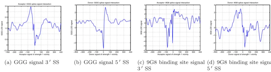
As an example of preferential motif location, we present in Figure 11 Logarithm of Odds (LOD) diagrams we measured in the vicinity of SSs for two known ISE and ESE motifs, GGG [70] and (GAC)n/ACGAGAGAY/WGGACRA
(9G8 binding site) [62]. We calculate LOD diagrams as
the logarithm of the ratio of signal concentration near SS to the signal concentration near splice-like signal [see Sec-tion Using detected signals to improve SS prediction]. The sig-nals have distinct bell-shaped concentration increase or decrease once we are getting closer to SS.
Our signal-detecting framework is purely based on Hid-den Markov Models (HMM). HMM has many attractive properties in the context of motif detection, such as a trac-table probabilistic inference and learning procedure, flex-ible topology, and ability to incorporate prior knowledge.
Using the mixture of Hidden Markov Models
Our strategy of motif detection is based on clustering with Mixture of Hidden Markov Models (MHMM). MHMM has a long record of successful implementations that started in speech recognition [71] and later were used for clustering protein families [72] and sequences [73]. To simulate location constraints of motifs within mRNA we use convolution of geometric states, that is described with bell-shaped negative binomial distribution, characterized by parameters p (probability to stay in the same state) and n
(number of consecutive states in convolution) [74]. To detect motifs we fit our MHMM model, shown in Figure 12, to the set of sample sequences, using the Baum-Welch algorithm described in [75,76]. The mixture component, shown in Figure 12, is a Hierarchical HMM (HHMM) with stack transformation to a plain HMM, as described in [77].
Many contemporary motif finders [63,67] use Product Multinomial (PM) model [65]. PM model corresponds to the widely known binding motif consensus, which could be easily visualized with logos [78]. The HMM motif model is strictly more general than the standard PM model, since the HMM model is capable of catching dependencies between adjacent motif positions, which LOD diagram for GGG signal, reported as an ISE (Figures 11(a), 11(b))
Figure 11
LOD diagram for GGG signal, reported as an ISE (Figures 11(a), 11(b)). LOD diagram for 9G8 signals, reported as an ESE (Fig-ures 11(c),11(d))
−400 −300 −200 −100 0 100 200 300 400
−0.5 0 0.5 1 1.5 2 2.5 3 3.5
Acceptor−GGG splice signal interaction
Acceptor signal of strength 1 vicinity
GGG LOD signal
(a) GGG signal 3SS
−400 −300 −200 −100 0 100 200 300 400 −3
−2 −1 0 1 2 3
Donor−GGG splice signal interaction
Donor signal of strength 1 vicinity
GGG LOD signal
(b) GGG signal 5SS
−400 −300 −200 −100 0 100 200 300 400 −6
−5 −4 −3 −2 −1 0 1 2 3 4
Acceptor−9G8 splice signal interaction
Acceptor signal of strength 1 vicinity
9G8 LOD signal
(c) 9G8 binding site signal 3SS
−400 −300 −200 −100 0 100 200 300 400 −3
−2 −1 0 1 2 3
Donor−9G8 splice signal interaction
Donor signal of strength 1 vicinity
9G8 LOD signal
used to be a major improvement to weight matrices (PM model) [52]. Furthermore, a mixture of HMMs is poten-tially able to recognize dependencies between nonadja-cent positions, by subdividing motif families into several subfamilies, each catching a specific group of dependen-cies between local positions.
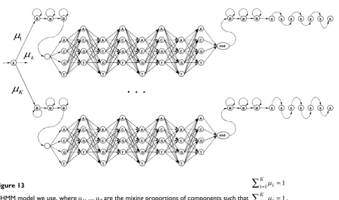
By implementing the MHMM topology, as shown in Fig-ure 13, we simultaneously learn competing HMM compo-nents of the mixture, so that they pick various competing motifs. Our application MHMMotif picks signals even if their observation frequency is low compared to simple background, i.e. a statistically significant concentration of a certain signal is not a primary detection criteria. Internal signal structure and its preferential location are the main conditions for our tool. This is another advantage of our approach compared to existing methods.
Since prediction of SS enhancing elements is still an active research topic, we decided to supplement the known enhancing motifs [see Subsection Splicing signals] with newly discovered putative enhancers. Our initial assump-tions of motif finding capability of MHMM were sup-ported by successful preliminary test results on artificial data sets, where known SF2/ASF [79] and SC35 [80] ele-ments were detected against random background. Another experiment on the sample set of 1,871 human promoter segments (-150...+10 bps relative to initial codon) from The Eukaryotic Promoter Database [81], clearly identified known landmarks of this area, such as OCT-1, NF-1 and AP-2 factors in addition to TATA-box, CAT-box, GC-box and TATA-like A-box factor. Having pre-liminary-encouraging results, we applied MHMMotif tool
to the splicing data sets [see Subsections Detection of ISE signals and Detecting ESE signals].
Using detected signals to improve SS prediction
Found ESE and ISE motifs have been evaluated for the ability to improve SS prediction with our new splicing simulator SpliceScan. Our splicing model is based on var-ious-strength SS interaction with signals, such as SS them-selves, and Enhancing/Silencing motifs located nearby.
SS classification enhancement in our system follows Baye-sian rule in terms of Logarithm of ODds ratio (LOD) [82]
The quantity Prob(D|H) is called the likelihood of the data
D (in our case ISE, ISS, ESE, ESS and competing SS signals) under hypothesis H. The last term of (4) is the LOD ratio of the prior probabilities of the Splice versus Splice-like signals, obtained with the Bayesian sensor. The first sum term in (4) takes into account the evidence provided by the data and comes up with a valid posterior LOD ratio. In order to make a noise-tolerant conversion of donor and acceptor probabilistic sensor scores into prior LOD, we approximate real signal score distribution histograms with a mixture of Beta Probability Density Functions (PDFs). The PDF of the Beta distribution is
and the mixture of n components is
LOD ob D H ob D H
ob
i
n i
SS i
SS
= ⎛ ⎝
⎜⎜ ⎞⎠⎟⎟ +
= ¬
∑
log ( | )( | ) log
(
( ) ( ) 1
Pr Pr
Pr HH ob H
SS SS
)
( )
Pr ¬ ⎛ ⎝
⎜ ⎞
⎠
⎟ ( )4
Beta p a b a b
a b p p p
a b
( , , ) ( )
( ) ( ) ( ) ,
= Γ + − − − ≤ ≤ Γ Γ
11 1 0 1
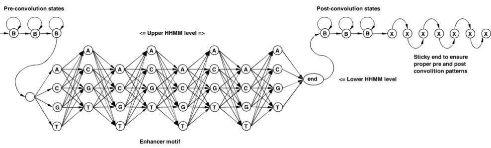
In our HHMM motif model B denotes background state – equiprobable emission of A, C, G, T
Figure 12
In our HHMM motif model B denotes background state – equiprobable emission of A, C, G, T. X is a special marker for sticky end handling to ensure proper convolution patterns. Sticky end of 10 X's is automatically added to every sample sequence by our tool.
B B B
A
C
G
T A
C
G
T A
C
G
T A
C
G
T A
C
G
T A
C
G
T A
C
G
T A
C
G
T
end
B B B X X X X X X X
Pre-convolution states Post-convolution states
Enhancer motif
Sticky end to ensure proper pre and post convolition patterns <= Lower HHMM level
. Using the Expectation Maximization algorithm for ture learning, as explained in [83], we fitted the beta mix-ture (5) to the donor and acceptor SS score histograms as shown in Figure 14.
The donor histogram (shown in Figure 14(a)) was fitted in the range from -25.1 to -0.38 with the mixture
Mixdonor(p) = 0.006 × Beta(p, 0.06, 0.91) + 0.994 × Beta(p,
14.27, 1.80)
and the acceptor histogram (shown in Figure 14(c)) was fitted in the range from -111.01 to -19.19 with the mixture
Mixacceptor (p) = 0.83 × Beta(p, 48.42, 6.37) + 0.17 × Beta(p, 7.18, 1.85)
where we assume probability argument in the formula
We then calculated the Cumulative Distribution Function (CDF) and subdivided the result probability into 10 equal intervals with corresponding average LOD scores as shown in Table 4.
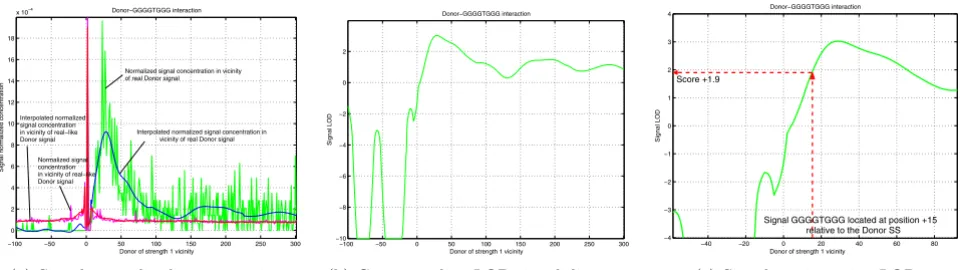
We built LOD diagram for each of the enhancing motif interacting with SS of different strengths (in range from 1 to 10), similar to shown in Figure 15. First, we measure normalized signal concentrations around SS, as shown in Figure 15(a). Using Matlab® polynomial interpolation we
approximated characteristics as could be seen in Figure 15(a). In order to find LOD characteristic, shown in Figure
15(b), we calculate , where
Prob(D|HSS) is normalized signal concentration at certain
location next to a SS and Prob(D|H¬SS) is normalized sig-nal concentration at certain location next to a splice-like signal. Signal LOD scoring happens as schematically shown in Figure 15(c).
We were not able to use all the available enhancing/silenc-ing signals for SS prediction. Part of the problem appears that the linear LOD sum accumulates noise and can only include limited number of factors. The signals we used for donor enhancement are all ISE elements supporting 5' SS shown in 7(h)-7(m), plus ESE element shown in Figure
Mix p qi Beta p a b q q i
n
i i i i i
n
( )= × ( , , ), ≤ ≤ , =
( )
= =
∑
∑
1 1
0 1 1 5
p
raw score range
range range range raw score
=
−
− ≤ ≤
min
max min , ifmin maax max
min
range raw score range
raw score range
,
, ,
, .
1 0
if if
> < ⎧
⎨ ⎪ ⎪⎪
⎩⎩ ⎪ ⎪ ⎪
log ( | )
( | )
2
Pr Pr
ob D H ob D H
SS
SS
¬
⎛ ⎝
⎜ ⎞
⎠ ⎟
MHMM model we use, where μ1, ..., μK are the mixing proportions of components such that
Figure 13
MHMM model we use, where μ1, ..., μK are the mixing proportions of components such that .
B B B
A C G T
A C G T
A C G T
A C G T
A C G T
A C G T
A C G T
A C G T
end
B B B X X X X X X X
B B B
A C G T
A C G T
A C G T
A C G T
A C G T
A C G T
A C G T
A C G T
end
B B B X X X X X X X X
1
μ
K
μ
k
μ
μi i K
=
∑
1 =1 μi i K=
8(a), 8(d), 8(g) and 8(j) combined with hnRNP A1, poly A and srp20 signals [see Subsection Splicing signals]. Sur-prisingly, polyadenylation signal use contributed substan-tial enhancement to the ROC diagram. We were not able to use SF2/ASF and SC35 enhancing signals for having LOD characteristics with indistinct enhancement profile. For acceptor enhancement we used ISE elements support-ing 3' SS shown in Figures 7(b), 7(c) and 7(e) plus ESE element shown in Figure 8(a), 8(d) and 8(g) combined with hnRNPAl, polyA and srp20 signals.
SS/SS interaction LOD diagrams are the key ingredient of our prediction algorithm as they contribute most to SS prediction enhancement. Figure 16 shows various interac-tion diagrams. X-axis is the SS vicinity posiinterac-tion, where SS of strength 1 located at 0, Y-axis is the strength of interact-ing signal and Z-axis is the LOD characteristic. The main conclusion we make based in Figures 16(a) and 16(b) is that weak signal preferentially avoids strong competitors nearby, especially inside exon, as they can redefine exonic boundary. Figures 16(c) and 16(d) indicate that weak sig-nal (donor or acceptor) has preferential need for strong complementing exonic boundary.
Donor and acceptor histograms approximated with a mixture of Beta distributions
Figure 14
Donor and acceptor histograms approximated with a mixture of Beta distributions.
−120 −10 −8 −6 −4 −2 0
20 40 60 80 100 120
(a) Donor histogram
0 0.1 0.2 0.3 0.4 0.5 0.6 0.7 0.8 0.9 1 0
1 2 3 4 5 6 7
Beta mixture approximation
0 10 20 30 40 50 60 70 80 90 100 0
50 100 150 200
(b) Donor histogram approximation
−900 −80 −70 −60 −50 −40 −30 −20 −10 20
40 60 80 100 120 140 160 180
(c) Acceptor histogram
0 0.1 0.2 0.3 0.4 0.5 0.6 0.7 0.8 0.9 1 0
2 4 6 8 10
Beta mixture approximation
0 10 20 30 40 50 60 70 80 90 100 0
50 100 150 200
Authors' contributions
AC, HA and IR conceptualized the project. AC imple-mented, learned and tested Bayesian sensor, SpliceScan and MHMMotif. HA and JD helped to design the SpliceS-can and MHMMotif tools, provided general support. AC wrote the manuscript. All authors read and approved the final manuscript.
Reviewers' comments
Reviewer's report 1Manyuan Long, Department of Ecology and Evolution, The University of Chicago Chicago, United States, Email: [email protected]
The authors attempted to develop a simple sensor to detect splice and splice- site signals. A 7-mer was designed to scan a sequence. The ROC diagrams (Fig. 3) showed its obvious advantage, significantly higher specificity and sensitivity than other methods. In addition, the authors also used MHMM to detect ISE and ESE signals and used found signals to improve SS prediction. I think that the authors developed useful new methods for SS detection and I favor its publication in Biology Direct. However, I
also have following minor concerns and hope them get fixed in revision.
Page 1: "Figure 1...": is not original, some sources should be cited (for example, the early work of Tom Schnider of NCI in 1992?". Originality is something that a paper in bioinformatics wants to emphasize.
Author response
For graphical representation of splicing motif consensuses we extracted multiple splicing motifs from our database and used WebLogo tool [78]to build the logos
Page 1: " the human transcribed region have plenty of motif....": it should be pointed out how are these motifs defined and why mentioned here? Is it relevant to the intron splicing?
Author response
Many oligonucleotides have composition identical to known potent splicing signals and at the same time are not supported by spliced alignment. Ab initio SSs prediction has to filter out such signals to predict the correct gene structure(s).
Page 2, the second paragraph, the caveat of current meth-ods to detect SSs is pointed out: non-coding exons do not have three-periodic coding components. The idea used is the signal interaction: SSs, ISE, ESE, ESS and ISS. New gene structural annotation tool SliceScan is developed and reported in this paper. SS sensor is the key and several majors SS sensors reviewed.
Page 3: in the proposal of a new sensor and compute P (7-mer and SS), why to choose the 7-(7-mer rather than 8-(7-mer or 6-mer should be explained. In addition, the sign – I guess is "non-ss" should be defined. If my guess is correct, this equation makes sense. Biology Direct is a journal for
Example of ISE signal interactions
Figure 15
Example of ISE signal interactions.
−100 −50 0 50 100 150 200 250 300
0 2 4 6 8 10 12 14 16 18
x 10−4 Donor−GGGGTGGG interaction
Donor of strength 1 vicinity
Signal normalized concentration
Normalized signal concentration in vicinity of real Donor signal
Interpolated normalized signal concentration in vicinity of real Donor signal
Normalized signal concentration in vicinity of real−like Donor signal Interpolated normalized signal concentration in vicinity of real−like Donor signal
(a) Signal normalized concentrations
−100 −50 0 50 100 150 200 250 300
−10 −8 −6 −4 −2 0 2
Donor−GGGGTGGG interaction
Donor of strength 1 vicinity
Signal LOD
(b) Corresponding LOD signal diagram
−40 −20 0 20 40 60 80
−4 −3 −2 −1 0 1 2 3 4
Donor−GGGGTGGG interaction
Donor of strength 1 vicinity
Signal LOD
Signal GGGGTGGG located at position +15 relative to the Donor SS Score +1.9
(c) Signal scoring using LOD
Table 4: Prior LODs
Strength Probability Prior donor LOD Prior acceptor LOD
1 0–0.1 -6.89 -9.10
2 0.1–0.2 -3.53 -5.65
3 0.2–0.3 -2.54 -4.51
4 0.3–0.4 -1.41 -3.69
5 0.4–0.5 -0.50 -2.84
6 0.5–0.6 0.01 -2.38
7 0.6–0.7 0.60 -1.86
8 0.7–0.8 1.06 -0.89
9 0.8–0.9 1.99 -0.26
general biology audience; not only for computational biologist so the jargons and special signs should be avoided or if having to use them, explanations should be given.
Author response
7-mer is the size of donor consensus minus GT dinucleotide, since it is always the same, as could be seen in Figure 1(a). For the modelling of acceptor signal 7-mer appears to be optimal: shorter oligonucleotide will have limited capability of represent-ing long-range positional correlations, while longer oligonucle-otides will produce large combinatorial table difficult to learn.
Page 7: I am not sure how they identify ISEs; section 3.2 is unclear. It seems the conservation is the only criterion. This might be reasonable in a narrow scale of evolution. But given the high evolutionary rate of intron sequence with a lot insertion-deletion (indels), I am suspicious of its feasibility because of the difficulty in alignments to identify the short homologous sequences. Although I do not oppose the approach, a cautionary note in the discus-sion should be given, which I think will be useful to col-leagues.
LOD diagrams for Donor and Acceptor signal interactions
Figure 16
LOD diagrams for Donor and Acceptor signal interactions.
(a) Donor-Donor interaction (b) Acceptor-Acceptor interaction
Author response
ISE signals are predicted using EM learning of MHMM model on intronic fragments of human genes. Main detection criteria used:
1. Close localization of putative signals to the intronic bounda-ries,
2. Constant size of putative enhancer,
3. Affinity of putative enhancing element to a certain HMM profile.
To test hypothesis of their higher conservation, compared to other oligonucleotides, we use mouse-rat intronic alignments that have substantial conserved domains.
Typo: Page 12: should be put in a different place to make reference continuous.
Reviewer's report 2
Arcady Mushegian, Stowers Institute, Kansas City, United States
Email: [email protected]
Good: 1. Part 2: the main idea appears to be to trade a more complex model for a larger training set. This seems to improve specificity of the splicing site detection.
Two relevant issues that are not discussed but should be: a. In Figure 3, all ROC curves are still below the non-dis-crimination line – is this acceptable.
Author response
We use ROC curve different from common True Positive Frac-tion vs. False Positive FracFrac-tion plot, where diagonal is a non-discriminant test result. In our test we know total number of positive cases, so we can build Sn vs. 1 - Sp curve, which is more informative for application comparison purposes.
b. Gain of the current method is more evident in the lower FP zone, where sensitivity is also low.
Author response
All application ROC curves converge to one point with 100% sensitivity and 0% specificity. The curves differ for lower sensi-tivity values, where we can speculate about prediction quality. Some applications, like NetUTR and ExonScan, have sensitiv-ity artificially limited to ~50%. Performance analysis for such applications makes sense only in lower sensitivity quarters.
2. A repertoire of intronic splicing enhancers was detected, which is interesting. Not so good: 1. Very unclear writing at different levels:
a. Various inconsistencies and poorly defined terms, for example on pg. 3–4, authors say that they compiled two test sets, and then describe three. Or on pg. 4, line 8 and further: what is "cross-correlating"?
Author response
Cross-correlation means the genes in learning and test set have extensive homologous regions, which favorably affects sensor performance on the test set and should be avoided for rigorous comparison.
b. section 3.1 : MHMM is not described well: we see a mix of introductory references on general HMMs, of more spe-cialized references that may be telling something relevant but we do not know that, and cat's cradle pictures which are not self-explanatory (and what about these mu param-eters?).
Author response
Here we try to reach reasonable compromise between complete system definition and skipping details of well known results from artificial intelligence community, which we reference. Please refer to MHMMotif application source code for more details.
2. The Results section mentions the programs that work less well than SpliceScan. But we do not hear about com-parison between SpliceScan (which barely gets over the non-discrimination line) and half a dozen other, more successful methods represented on the same plots. If the goal of the work was to improve the ab initio approach (cf a line in the abstract), this has to be maintained as the message throughout the paper.
Author response
Our method has clear advantage in case of 5' UTR gene frag-ment structural prediction according to ROC curves shown in Figures 9(e)and 9(f). In case of gene structural prediction in CDS area, one should use different application, such as GenS-can, since SpliceScan does not have frame-consistent synchro-nization component.
Overall, this manuscript reads more like the technical report on the ongoing project than a stand-alone paper.
I declare that I have no competing interests.
Reviewer's report 3
On "Method of predicting splice sites based on signal interactions" by A.Tchourbanov et al., submitted to "Biol-ogy Direct"
The problem of identification of donor and acceptor splic-ing sites is not new, but far from solved, whereas identifi-cation of sites regulating splicing (exonic/intronic splicing enhancers/silencers) has emerged relatively recently. Given the importance of both these problems for gene rec-ognition and understanding alternative splicing, any progress in this area is most welcome.
The authors attempt to address both problems in one framework of Bayesian analysis. They apply Bayesian sen-sors to detection of donor and acceptor splicing sites. The exposition in this part (section 2, pp. 2–3) contains sev-eral gaps. It is not clear how well the described approach of 7-mer counting with subsequent Bayesian weighting generalizes; in particular, it seems that the sensors will not accept a completely new 7-mer as a site. If the authors implicitly claim that all possible 7-mers have already been observed in the training set, and the only problem is proper weighting, this needs to be substantiated. A helpful piece of data would be the rank distribution of 7-mers in the positive and negative sets. How many 7-mers have been observed only once in the positive set (and would be missed if only half of that set were used for training)?
Author response
With cross correlation removed between learning set and the test set, when testing on the set of 250 human genes, we had miss rate of 0.52% for our 5'SS sensor, which is acceptably low value. For 3'SS sensor overall miss rate is negligibly low, since sensor topology is composite of several blocks. We show top 40 ranking 5'SS nonamers in Table 2. We added discussion on sensor performance related to learning set size [see Subsection
Learning set size study/, where we show that Bayesian sensor has preference for the large learning sets. For example, the sen-sor could be successfully applied to recognition of the Transla