Abstract A comprehensive database, containing biolog-ical and chembiolog-ical information, collected in the frame-work of the bilateral interdisciplinary MARS project (“biological indicators of natural and man-made changes in marine and coastal waters”) during the years 1995–1997 in the coastal environment of the North Sea, was subjected to a multivariate statistical evaluation. The MARS project was designated to combine a variety of approaches and to develop a set of methods for the em-ployment of biological indicators in pollution monitoring and environmental quality assessment. In total, nine ship cruises to four coastal sampling sites were conducted; 765 fish and 384 mussel samples were analysed for bio-logical and chemical parameters. Additional information on the chemical background at the sampling sites was derived from sediment samples, collected at each of the four sampling sites. Based on the available chemical data in sediments and black mussel (Mytilus edulis) a pollu-tion gradient between the selected sites, was established.
The chemical body burden of flounder (Platichthys fle-sus) from these sites, though, did not reflect this gradient equally clear. In contrast, the biological information de-rived from measurements in fish samples displayed sig-nificant a regional as well as a temporal pattern. A multi-variate bioindicator data matrix was evaluated employ-ing a factor analysis model to identify relations between selected biological indicators, and to improve the under-standing of a regional and temporal component in the pa-rameter response. In a second approach, applying the k-means algorithm on the data matrix, two significantly different clusters of samples, characterised by the current health status of the fish, were extracted. Using this clas-sification a temporal, and in the second order, a less pro-nounced spatial effect was evident. In particular, during July 1996, a clear sign of deteriorating environmental conditions was extracted from the biological data matrix.
Key words Bioindicators · Spatial pattern · Temporal pattern · North Sea
Introduction
One of the major challenges in environmental science is the integration of different measurements into an inte-grated view, to achieve a more general, reliable measure for the assessment of ecosystem health. The current re-search project was aimed at developing, from a combina-tion of biological parameters, a reliable tool for the as-sessment of environmental deterioration of coastal ma-rine ecosystems. Different biological parameters, rang-ing from biochemical tests at the molecular level to parasitological community parameters at the ecosystem level were included in the study. A summary of the pa-rameters under investigation is given in Table 1.
The project consisted of three biological sub-projects and addressed two topics: (1) the use of biochemical and histochemical biomarkers for biological effects monitor-ing; (2) the use of parasitological indices for biological S.R. Schmolke (
✉
) · E. JantzenGALAB, Max-Planck-Strasse, D-21502 Geesthacht, Germany
K. Broeg · G. Krüner · H. von Westernhagen
Alfred-Wegener-Institut für Polar- und Meeresforschung, Biologische Anstalt Helgoland-Notkestrasse 31, D-22607 Hamburg, Germany
S. Zander · W. Körting
Tierärztliche Hochschule, Bünteweg 17, D-30559 Hannover, Germany
V. Bissinger · P.D. Hansen
Technische Universität Berlin, Kepplerstrasse 4–6, D-10589 Berlin, Germany
N. Kress · B. Herut
Israel Oceanographic and Limnological Research Institute, P.O.Box 8030, Tel Shikmona Haifa, 31080, Israel
A. Sturm
UFZ-Umweltforschungszentrum Leipzig-Halle, Permoserstrasse 15, D-04318 Leipzig, Germany
Present address:
S.R. Schmolke, GKSS Research Center, Max Planck Strasse, D-21502 Geesthacht, Germany
O R I G I N A L A R T I C L E
S.R. Schmolke · K. Broeg · S. Zander · V. Bissinger P.D. Hansen · N. Kress · B. Herut · E. Jantzen G. Krüner · A. Sturm · W. Körting
H. von Westernhagen
Multivariate statistical approach to the temporal
and spatial patterns of selected bioindicators observed
in the North Sea during the years 1995–1997
effects monitoring. Environmental chemistry was added as a third supplementary activity. For a detailed descrip-tion of the specific tasks, methods used, and results of each sub-project the reader is referred to Bresler et al. (1999), Broeg et al. (1999), and Kress et al. (1999) in this issue.
Since an attempt at an integrated evaluation of data was initialised only after the termination of the experimental work, the statisticians had no influence on experimental planning and data management. Hence the specific require-ments for a multivariate analysis were not considered dur-ing the experimental planndur-ing and execution. In particular, the lack of consistency in the data matrix in time and space turned out to be a major disadvantage for evaluation.
The focus of the evaluation was, on the one hand, on identifying existing relations between the biological pa-rameters under investigation and, on the other, on assess-ing the possible dependence of the multivariate bioindi-cator pattern on a spatial and temporal scale. Due to the above-mentioned drawbacks in co-ordinated planning, a multivariate analysis could only be applied to a limited set of data.
Materials and methods
From 1995 to 1997 nine sampling campaigns were conducted in the North Sea (2×winter, 2×spring, 2×summer, 3×autumn). In all
figures as well as in the text the campaigns are identified by a four-digit number. The first two digits stand for the year, the sec-ond two for the month of the sampling campaign. Flounder sam-ples were collected at three, and in 1997 at four sites (Fig. 1). To avoid undesired age and size effects, only fish samples of a nar-row size range (18–25 cm total length) were included in the analysis. The initial working hypothesis on which the sampling design was based was the assumption of a pollution gradient among the chosen sites which was expected to be reflected by the bioindicator response. The assumed pollution gradient, was Table 1 Summary of
parame-ters under investigation. The parameter abbreviation (ParameterAbb), the full name (ParameterFull), the unit, and the responsible institute: BAH (Biologische Anstalt Helgo-land), THH (Tierärztliche Hochschule Hannover), TUB (Technische Universität Berlin), IOLR (Israeli Oceano-graphic and Limnological Research Ltd.)
ParameterAbb ParameterFull Unit Origin
dddfat DDD µg/kg liver fat BAH
ddefat DDE µg/kg liver fat BAH
ddtfat DDT µg/kg liver fat BAH
dieldrinfat Dieldrin µg/kg liver fat BAH
ERO EROD activity nmol min–1mg–1 (Protein) BAH
gHCHfat Hexachlorocyclohexan µg/kg liver fat BAH
HCBfat Hexachlorobenzene µg/kg liver fat BAH
Len Length cm BAH
LiC Liver colour 1–6 BAH
LiF Macrophage aggregate lipofuscin Mean absorbance BAH
LY1 Lysosomal stability 1 min BAH
LY2 Lysosomal stability 2 min BAH
MAA Macrophage aggregate area µm2 BAH
MAM Macrophage aggregate activity Mean absorbance BAH
Mat Maturity 0/1 BAH
nLi Neutral lipids liver Mean absorbance BAH
ocsfat Octachlorstyrol µg/kg liver fat BAH
pentBENZfat Pentachlorobenzene µg/kg liver fat BAH
Sex Sex 1,2 BAH
sPCBfat Sum polychlorinated biphenyls µg/kg liver fat BAH
Cd Cadmium µg/g (wet.wt.) IOLR
Cu Copper µg/g (wet.wt.) IOLR
Fe Iron µg/g (wet.wt.) IOLR
Hg Mercury µg/g (wet.wt.) IOLR
Mn Manganese µg/g (wet.wt.) IOLR
relDryWt Relative dry weight % IOLR
Zn Zinc µg/g (wet.wt.) IOLR
AnzArten Sum of species (parasite) In total 33 species THH
AnzahlHeteroxen Sum heteroxenic parasites In total 22 species THH AnzahlMonoxen Sum monoxenic parasites In total 11 species THH ChE Cholinesterase activity nmol min–1mg–1 (protein) TUB
DNA DNA unwinding –log F TUB
GST Glutathione-S-transferase activity nmol min–1mg–1 (protein) TUB
Fig. 1 North Sea sampling sites. The fish sampling sites are
arranged in the order: Elbe river mouth (ElbM, CuxL), polluted, Eider river mouth (EidM, EidS), moderately polluted and Tiefe Rinne Helgoland (TieR, HelD) control site. With regard to the hydrographic conditions at the other stations the TieR site was unfortunately not directly comparable to the other sites due to its higher salinity and greater depth. Thus in 1997 it was agreed that another unpolluted site off the island of Spiekeroog (Spie, SpiW) should be sampled.
In principle, the evaluation of an environmental database con-taining a temporal and a spatial dimension can be approached at different levels of detail. Assuming a significant pollution gradient between sampling sites calls for an evaluation based on sites. The means of sensitive parameters grouped by sites should reflect the pollutant gradient as a region-dependent response. Yet an effect becomes visible only when it is not superimposed by other effects that are not dependent on the sampling region, such as seasonal ef-fects or efef-fects caused by the current state of the reproductive cy-cle of the test organisms. Also the migratory habit of fish is ex-pected to disturb the pattern of biological responses observed in hauls from distinct sites. In order to extend the evaluation of a database on temporal effects, differentiation not only at a spatial level but also at temporal levels is needed. Thus the number of cases to be considered will increase from 3 (three stations) to 27 (3 stations × 9 campaigns). Although this approach will yield a more detailed analysis, extended by the temporal dimension, it will also provide averaged information. The total information con-tained in the database is considered only by applying a specimen-based approach. Here the individual biological functionality of each analysed individual is taken into account, and a large variety of biological factors that may influence the response of each indi-vidual are under discussion. For example, the migratory habit of fish may influence the composition of a haul at a given site. Since the migratory history of the fish is uncertain and may influence the range of variability of the biological and chemical parameters, there are good reasons to use a statistical approach at the individu-al level in order to minimise any loss of information rather than to conduct an evaluation at a more general level.
Two multivariate approaches are discussed in this paper. First, a factor analysis has been performed to examine relations between the parameters (bioindicators) and to elaborate initial information about dominant effects on a regional and temporal scale. Always when the term significant is used in the discussion, a P value low-er than 0.05 is implied. An ovlow-erview of the multivariate statistical methods applied is given in Dillon and Goldstein (1984) or Henrion and Henrion (1994). The factor analysis is an exploratory method to identify structures in multivariate databases by the re-duction of the original multiple variables system to a simpler system with a reduced number of superimposed complex variables (factors). The aim is to condense the information from a multivari-ate data matrix to a less complex system to facilitmultivari-ate interpreta-tion. The successful application of this method to environmental multivariate databases is described in several recent publications. The method has been used to describe regional water quality (Reisenhofer et al. 1996) or to identify pollution sources in marine (Naes and Oug 1997) and river systems (Götz et al. 1998). Factor analysis was also used to assess biological systems, for instance the identification of flat fish species by means of morphological characteristics (Piet et al. 1998). The second multivariate method used successfully to discover structures in the present data matrix was the k-means clustering method. In contrast to the factor analy-sis, which combines information from individual parameters to factors, the k-means cluster method groups individual objects (fish samples) into clusters of similar characteristics (parameter pattern). This method is based on an algorithm developed by MacQueen (1967). The algorithm separates the data matrix into a pre-defined number of clusters. The objective of the sorting crite-rion is to achieve a minimum of variance within clusters and a maximum between clusters. As was the case for the factor analy-sis, this method has been applied in recent studies on environmen-tal databases to assess the water quality in the river Elbe (Götz et al. 1998). The analyses were performed using Statistica v.5 (Stat-soft Inc.).
A specific advantage of the present project database was that work was done on only one fish species, the flounder (Platichthys
flesus). This allowed a direct comparison between individuals
making use of the different biomarkers under investigation. Fur-thermore, an important requirement for a successful multivariate approach at the specimen level was a high level of consistency in the used data matrix. Unfortunately, none of the 764 fish samples was analysed for the entire set of relevant parameters. Thus the number of parameters that could be considered for the multivariate statistical analyses was a compromise between maximising the number of included parameters, on the one hand, and maximising the number of individual fish that were sufficient as characterised by the selected parameters, on the other. The criterion for includ-ing a parameter was the frequency of measurements and the ability of combinations with as many parameters as possible in the same individual. This was the reason why results from the chemical an-alyses were not included in the multivariate calculations. The con-sideration of these parameters would have decreased the total number of valid cases (fish specimens) below an acceptable value. Although there are some suitable methods for modelling gaps in a data matrix, they all increase the uncertainty of the results, and they should only be applied if there is a good understanding of the parameter response characteristics. It was decided to exclude all samples with missing values. This pre-condition meant that fewer samples were considered and led to a loss of information from the entire database. But the probability of lost information from the reduced data matrix was accepted to avoid artificial results by re-placement of missing data by extrapolated values. On the basis of these prerequisites the following parameters were incorporated in-to the multivariate analysis (detailed descriptions of the parame-ters and applied methods are given in the respective references):
Macrophage aggregate area (MAA), the mean size of macrophage aggregates in flounder liver (Broeg et al. 1999).
Macrophage aggregate activity (MAM), the activity of acid phos-phatase in macrophage aggregates of flounder liver (Broeg et al. 1999).
Lysosomal stability (LY2), the membrane stability of hepatocyte lysosomes (second group of lysosomes displaying an early mem-brane break down) (Broeg et al. 1999).
EROD activity (ERO), the activity of cytochrome P450 dependent monooxygenase Ethoxyresorufin-O-deethylase (EROD) (Broeg et al. 1999).
Choline esterase activity (CHE) (Bressler 1999).
Number of parasite species (ANZARTEN) (Broeg et al. 1999). Liver colour (LIC), a parameter that represents the pathologically induced lipid accumulation in flounder liver (Broeg et al. 1999).
In addition to the biological investigations a limited number of chemical analytical data from fish, mussels and sediment samples were available. The respective samples were used for orientation as regards chemical pollution at the different sites, because the number of analytical data points for environmental chemistry was not sufficient to include them in the multivariate statistical analy-sis.
Results
ac-tivities. The fourth sampling site, Spie, thought to be an alternative unpolluted reference site, was only used dur-ing the last year of sampldur-ing and could not be included in all analyses due to the lack of sufficient data.
Characterisation of the sampling sites by chemical pollution burden
Sediments
A look at the heavy metal burden in sediments supports the pollutant gradient assumption made above. Figure 2 dis-plays the dry-mass-related heavy metal content in sediment samples taken during the cruises in April and October 1996. To permit an overview of all heavy metal values in one single graph, concentrations are standardised for each element by its overall mean concentration from both cam-paigns and all sites [Std. score=(raw score/mean (all sam-ples)]. The observed concentration values of each sample could be recalculated by multiplying each displayed single value by the mean concentration of the related element giv-en in the figure leggiv-end. A trace elemgiv-ent gradigiv-ent betwegiv-en the chosen sites is obvious from the graph. The observed heavy metal burden of the sediment samples is consistent with the assumption of a pollution gradient between the chosen sampling sites.
The same ranking had been obtained on the basis of polyaromatic hydrocarbon (PAH) determination in the sediments of the three sampling sites. PAH concentra-tions that had been determined in the sediment samples of the sites were: 5, 40 and 100 µg/g dry weight at TieR, EidM, and ElbM, respectively. Due to the limited num-ber of samples for the residue analyses from the sedi-ments though, data have not been subjected to statistical treatment.
Black mussel
Close to the fish haul sites, mussel samples were also taken. During two campaigns 60 mussel pools were col-lected at four sites and analysed for their heavy metal burden in soft tissue. In general the same gradient was found as for the sediment samples. In Figs. 3 and 4 the cadmium and copper burdens of all available mussel samples are displayed. Each box (site/cruise grouped) contains 5–10 values. The directly comparable median concentration values observed at each site during the same cruise are connected by dashed lines. In particular Cd and Cu, elements which are correlated mainly to an-Fig. 2 Standardised heavy metal concentration per dry weight in
sediment. Each element is characterised by two data points (sym-bols), one for each campaign, which are connected by lines. To en-able direct comparison between different elements, all element values are divided by their overall mean concentration, which is given in the legend in square brackets
Fig. 3 Cadmium concentration in mussel soft tissue per wet
weight, grouped by site and campaign. Each box indicates: mini-mum, maximini-mum, median, 25%, 75% quartile, 95% confidence in-terval (notch)
Fig. 4 Box and whisker plots of the copper concentration in
mus-sel soft tissue per wet weight, grouped by site and campaign. Each
box indicates: minimum, maximum, median, 25%, 75% quartile,
thropogenic emissions, display a similar pattern. During both the spring and autumn 1997 campaigns, the CuxL (close to ElbM) site showed significantly elevated val-ues. But not only a spatial difference was obvious. A sig-nificant temporal effect was also seen [analysis of vari-ance (ANOVA)]. At all sites the highest mean heavy metal burden was detected in autumn 1997. In the case of Cu a factor close to 2 was observed between the two campaigns at the CuxL site.
Flounder
Heavy metals were measured in five fish samples from two campaigns at all three sampling sites. Organic
pollu-tants were determined during three other campaigns, in 4–11 samples from each site. Unfortunately, no individu-al fish sample was anindividu-alysed for both heavy metindividu-als and organic pollutants.
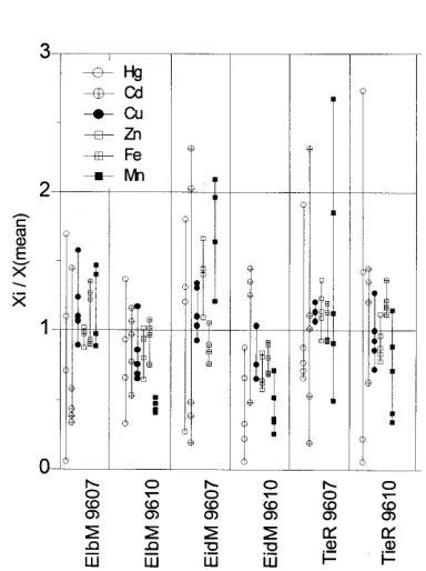
The heavy metal burden of flounder tissue is shown in Fig. 5. To gain an overview of all elements in one figure, the displayed concentrations were standardised on the basis of the mean element concentrations from all samples. To enable the recalculation of the element concentrations of all samples, means as well as the site/campaign means and standard deviations of the ele-ments are summarised in Table 2. There was no apparent spatial effect. During both the summer and autumn 1996 campaigns, no significant (ANOVA) differences in the heavy metal burden (except Fe) of flounder from the three sites were found. Only a temporal effect could be determined in the case of Cu, Mg and Zn, indicating higher contamination with the three metals in July than in October.
A spatial effect of heavy metal burden was best ascer-tained in the sediment samples and in the residues from mussel soft tissue. For fish muscle contamination, though, no clear spatial gradient was apparent, yet a tem-poral effect could be shown. Due to the limited numbers, results derived from the chemical analysis should be viewed with the necessary caution.
Temporal and spatial pattern in the bioindicator database
Both spatial and temporal effects were present in the bio-indicator data matrix. The MAA will serve as an exam-ple for a campaign-dependent parameter (Fig. 6), and the lysosomal stability as a campaign- and time-dependent parameter (Fig. 7). Both parameters are displayed in sim-ilar plots where each data point gives the mean site/cam-paign value. The time-dependent nature of the parameter is best illustrated in the lower (B) plots. Here all mean site values are connected by single lines on a time (x) axis. Both parameters are characterised by significant (ANOVA) temporal patterns. The spatial trend of the pa-Table 2 Means and standard deviation of heavy metal concentration in Flounder (P. flesus) muscle tissue [µg/g (wet weight)]
Hg Cd Cu Zn Fe Mn
Means SD Means SD Means SD Means SD Means SD Means SD
9607 0.013 0.013 0.013 0.010 0.34 0.07 6.69 0.38 5.08 0.93 0.57 0.13
ElbM
9607 0.040 0.044 0.022 0.021 0.33 0.05 9.74 1.42 3.98 0.48 0.82 0.17
EidM
9607 0.018 0.010 0.021 0.017 0.33 0.02 7.94 1.13 4.58 0.59 0.65 0.40
TieR
9610 0.014 0.007 0.019 0.005 0.24 0.06 5.99 1.00 4.27 0.54 0.21 0.02
ElbM
9610 0.008 0.006 0.025 0.008 0.22 0.05 4.82 0.81 3.58 0.47 0.20 0.08
EidM
9610 0.016 0.022 0.024 0.007 0.28 0.06 6.30 0.91 5.41 0.43 0.32 0.15
TieR
All 0.018 0.022 0.021 0.012 0.29 0.07 6.91 1.83 4.48 0.83 0.46 0.30
groups
Fig. 5 Standardised heavy metal concentration per wet weight in
rameter is best reflected by the upper (A) plots. The three sites are collected under individual lines for each campaign. The x axis is a regional scale with increasing pollution expected from left to right. The trend of lower LY2 values, indicating higher pollutant burden at the ElbM site, is consistent over all cruises, and in the same range as the temporal effects. In contrast, the MAA pa-rameter shows no significant spatial trend (ANOVA).
In the following discussion two multivariate ap-proaches will be presented. In a first step the relations between selected bioindicators will be examined on the basis of the results of a factor analysis. In the second step it is attempted to distinguish between cam-paigns/sites of different disturbances by assessing the re-sults of a k-means cluster analysis. Seven parameters (MAA, MAM, LY2, EROD, LIC, CHE, ANZART) were subjected to multivariate investigations.
Of a total of 764 samples, only 274 were consistently examined for all selected parameters. An additional number of cases had to be rejected due to a high number of 0 values. In particular the MAA and MAM parameters were concerned when no macrophage aggregates could be found in the piece of liver examined. It is not clear yet whether this represents a real effect. Thus these samples
were excluded from the calculations. In the end, 136 cases were considered.
Two factors with eigenvalues greater than 1 were ex-tracted (Table 3). These two factors were able to explain 46% of the total variance. The factor loading is shown in Fig. 8. Factor loading can be interpreted as correlation between the respective variables and factors. The values contain information about the extent to which the factor determines the variables. The parameters LY2 and ANZARTEN dominate factor 2. Both parameters act in the same direction (positive loading) and contribute only in a minor way to factor 1. Factor 1 is primarily based on the MAA, LIC and CHE parameters. Whereas LIC and Fig. 6 Site and campaign grouped macrophage aggregate area
[µm2] mean values. Spatial trend plot (A) and temporal trend plot
(B). Increasing pollution burden at the different sites is expected in the order ElbM, EidM, TieR
Fig. 7A,B Site and campaign grouped mean values of lysosomal
stability (LY2). Spatial trend plot (A) and temporal trend plot (B). Increasing pollution burden at the sites is expected in the order ElbM, EidM, TieR
Table 3 Eigenvalues and explained variance of factor analysis
model. Rotation method Varimax. Only factors with eigenvalues greater then 1 are listed. Seven variables and 136 cases were in-cluded
Factor Eigenvalue % Total Cumulative Cumulative variance eigenvalue %
1 1.76 25.16 1.76 25.16
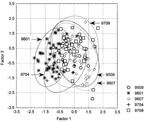
MAA are well correlated and are located close together with positive factor 1 loading, the CHE parameter func-tioned in the opposite direction. The contribution of MAM and EROD activity to the factor model was less pronounced and not specific to either of the two factors. The computed factor scores are displayed in Figs. 9 and 10 in scatter plots. Both plots display the same spread of data points in the two factor plane, which are calculated from the same factor model. Each grouping criterion, site and campaign, is marked individually in both figures. For better orientation all grouped data points are indicat-ed by 95% confidence ellipses. The calculatindicat-ed ellipses were based on the assumption that the two factors follow the bivariate normal distribution. The orientation of the ellipse was determined by the sign of the linear correla-tion between the two factors (the longer axis of the el-lipse was superimposed on the regression line).
A detailed elaboration of the factor analysis led to the following results. The sampling sites were only distin-guished by factor 2 (Fig. 9). Whereas most Elbe river (ElbM) data points were indicated by negative factor 2 values, the Eider (EidM) and Tiefe Rinne (TieR) sites were in the upper part of the graph, at positive factor 2 values. Factor 1 did not contribute to the separation, as it was reflected by the normal scatter of all different data points over the horizontal scale.
The temporal effects were analysed in the same way as the regional ones. To a certain extent the formulated factor model was also able to separate the sampling cam-paigns. Analysing the data point clouds in Fig. 10, the separation of cruise 9601 from 9607/9509 became obvi-ous. The 9607/9509 data points were located in the right half, the 9601 data points in the left half of the graph. The temporal distinction was based mainly on factor 1. The contribution of factor 2 to a separation of the cam-paigns was only poor.
A combination of the information of Fig. 8 and Figs. 9/10 gives an insight into the relations between the ob-served parameters and their site/campaign dependency. This is demonstrated on the fish samples which
originat-ed from the ElbM site in 9607. The ElbM observations are mainly found at low factor 2 values in the lower part of Fig. 9. Factor 2 itself was positively correlated and greatly influenced by the ANZARTEN and LY2 parame-ters (Fig. 8). During the 9607 campaign the factor 1 val-ues were mainly positive and thus they are concentrated in the right part of Fig. 10. Factor 2 was negatively cor-related with CHE and positively corcor-related with LIC and MAA (Fig. 8). In summary, the fish situation during the 9607 cruise at the ElbM site was characterised by elevat-ed MAA and LIC values and relevat-educelevat-ed ANZARTEN, LY2 and CHE values. This may point to an impaired health Fig. 8 Factor loading in a Varimax rotated co-ordinate system
Fig. 9 Fish samples in the factor score co-ordinate system
sepa-rated by site: 95% confidence area ellipses surround the observa-tions for each sampling site
Fig. 10 Fish samples in the factor score co-ordinate system
situation of the fish analysed in the Elbe estuary in the summer of 1996.
In general, determination of the parameter variability by the applied factor model was only weak (less than 50% explained variability) and thus the interpretation should be viewed with the necessary caution.
On the basis of the results from the factor analysis, the idea of using the second multivariate approach to an-alyse the data matrix without any assumption of a spatial or temporal structure in the database was employed. Re-gardless of the site or the haul from which the fish sam-ple originated, a k-means analysis was assessed by the pattern of the biological information available. This analysis (a special kind of cluster analysis with a pre-defined number of extracted clusters) was used to sepa-rate two groups of individuals from the entire pool of samples. The mathematical algorithm for this procedure works like a reversed analysis of variance. The clusters are created by grouping the samples, following the crite-rion of minimising the within-group variance and max-imising the between-group variance. It was tested wheth-er it would be possible to separate two groups, a clustwheth-er of fish with poor health and a cluster of less impaired in-dividuals.
For this analysis the same parameters as used for the factor model were considered. Prior to the analysis the data matrix was z-transformed (standardised on a param-eter mean value 0 and standard deviation 1).
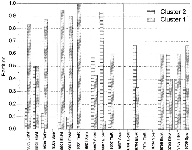
From this matrix it was possible to extract two obvi-ous different clusters. Cluster 1 contained 95 and cluster 2, a total of 115 cases (fish specimens). All mean param-eter values were significantly (ANOVA) different be-tween the extracted clusters, except the parasitological one (ANZARTEN) (Table 4). However, the ANOVA re-sults should be viewed with caution. When applying the test to clustered (sorted) objects this was not tested a pri-ori, and the results were capitalised on chance by arrang-ing the most statistically significant ANOVA’s possible. The pattern of the mean parameter values in each cluster is shown in Fig. 11. Each of the two clusters is displayed as a separate line connecting the standardised mean pa-rameter values. Cluster 2 shows a papa-rameter pattern which could be classified as a group of impaired individ-uals. The amplitude of all parameters indicates a bad health situation. In contrast, cluster 1 contains samples of unimpaired or less impaired individuals. At this point it should be emphasised again that the separation of the two clusters was based only on the parameter pattern of
the samples. In the next step it was tested how the sam-ples related to one of the two clusters were spread over the sampling campaigns and sites. Figure 12 shows the partitioning of samples classed in cluster 1 and 2, grouped by sampling site and campaign. Each bar indi-cates the partitioning of fish samples belonging to one of the two separated clusters. In total, the values of clusters 1 and 2 add up to 1 for each campaign/site. A strong temporal effect on the classification of the fish is obvi-ous. The most pronounced differences were found during the 9601 cruise when only 6% of the samples were classed as cluster 2 (impaired) and 94% as cluster 1 (un-impaired), and the 9607 cruise with a cluster 2/1 ratio of 67%/33%. It is not yet clear whether this obvious differ-ence is due to varying environmental pressure or rather dominated by the seasonal dependence of the response. However, a comparison of the 9607 (summer) cruise with the two available autumn cruises 9509 (cluster 2/1, 28%/72%) and 9709 (cluster 2/1, 47%/53%; the Spie site is not considered) showed a similar situation. Here as well, only the 9607 samples showed a clear preponder-ance of fish samples classified as cluster 2. Comparing all samples taken at the EidM sites only, the 9607 cruise is the only one in which the number of fish in cluster 2 predominates. Combining all this information, there is a strong indication that it can be assumed that during this period a major pollution event may have taken place that had influenced the health of the fish considerably.
Shifting the focus to the regional effect, a surprising-ly clear pattern was found. A comparison of the site ranking by cluster 2 partitioning led to a consistent pic-ture. During all cruises, irrespective of the season, the ElbM site displayed the highest fraction of cluster 2 Table 4 k-Means clustering
results: significance test of the separated clusters. P levels for the separation of cluster 1 and 2
Parameter P
LIC 0.000
MAA 0.000
MAM 0.000
LY2 0.000
ERO 0.000
CHE 0.000
ANZARTEN 0.286
Fig. 11 k-Means clustering results. Parameter mean values of the
samples, followed by the EidM and TieR sites. This or-der of sampling sites, the highest fraction of impaired fish samples at the ElbM site, the lowest at the TieR site, corresponded surprisingly well with the results of the chemical investigations, which produced the same ranking of sites.
Consistent with the results of the factor analysis ap-proach described above, both effects (temporal and spa-tial) were observed. It was also evident that the separa-tion of fish samples into unimpaired specimens at the reference site (TieR) and impaired individuals at the pol-luted sites was not possible. In particular during the 9607 campaign a notable fraction of impaired fish samples was observed at the supposedly cleaner control site TieR at Helgoland. This means that although the expected gra-dient in fish health was reflected by the site grouped samples, the clean site TieR and also the later-selected Spie site (9709) did not guarantee an undisturbed refer-ence fish sample.
Conclusion
In the present study, uni-, bi- and multivariate statistical relationships were examined between different types of biomarkers in flounder, in order to be able to associate them with pollution effects. While the individual param-eters have been discussed in detail in other contributions in the present volume (Bresler et al. 1999; Broeg et al. 1999; Kress et al. 1999), the primary aim of the present paper was to compare the various biomarkers in their suitability for the assessment of coastal water pollution. In addition, statistical analyses of the data sets of chemi-cal parameters were employed to classify the pollution status of the three main sampling sites.
Although the database for the calculation of multivar-iate statistics had some serious shortcomings in terms of completeness of the data matrix, the factor analysis and the k-means analysis enabled us to demonstrate a pollu-tion gradient between the three stapollu-tions Tiefe Rinne Hel-goland (TieR) < Eider river mouth (EidM) < Elbe river mouth (ElbM). The existence of a pollutant gradient be-tween the sites was supported by the chemical data from sediments and mussel tissue, but not by those measured in fish tissue. Due to the limited number of analyses, a temporal effect was not discernible.
The biological data displayed a temporal and a spatial pattern. To a certain extent, the biological indicators sup-ported an environmental pollution gradient between the chosen sites. Most parameters, though, showed a statisti-cally significant temporal pattern. The sampling locations Elbe river mouth (ElbM), Eider river mouth (EidM) and Tiefe Rinne Helgoland (TieR) were not sufficiently charac-terised by virtue of their spatial separation in order to clas-sify fish samples as impaired or unimpaired individuals. Although a regional effect was evident, it was of secondary importance and may have been blurred by the migratory activity of flounders from the Elbe estuary into the deeper areas of the German Bight (i.e. Helgoland Tiefe Rinne) in winter. Temporal effects were predominant, particularly between the end of 1995 and the summer of 1996, when the health of the system had deteriorated alarmingly. In 1997 all sites were still impacted, even though a pollution gradient between the sites could be observed. These find-ings were well in line with a pollution event that had been documented by other authors employing biological moni-toring exercises (Westernhagen and Dethlefsen 1997) dur-ing the same period in the German Bight. This event had been ascertained through the discovery of a considerable input of environmental chemicals (notably DDT) at the end Fig. 12 Partitioning of fish
of 1995 and the beginning of 1996 (ARGE Elbe 1997) (see also Broeg et al.1999, this issue), which apparently has had a dramatic effect on the health of the whole ecosystem in the German Bight.
Thus, as has equally been demonstrated by van der Oost et al. (1997) for freshwater lakes, it could be estab-lished that multivariate analysis is well suited to examine relationships between exposure to pollutants and the re-action of biochemical and community parameters in a marine ecosystem. In our study we were able to demon-strate the importance of biological effects monitoring for the detection and classification of pollution gradients, between differently impacted sites in the German Bight. All of the evaluated biomarkers had a certain potential to indicate ecosystem stress; yet for the improvement of marine ecosystem health assessment a validation of the ranking of the chosen indicators would be important.
Acknowledgements The authors wish to thank the German Min-istry of Education and Research (BMBF) for financial support. We thank Prof. Schöttler from the Project Management Organisation Biology, Energy and Environment (BEO), Helmut Bianchi from the International Office at the GKSS Research Centre, and the Joint Advisory Committee (JAC) for their advice and project co-ordination.
References
ARGE Elbe (1997) 20 Jahre Arbeitsgemeinschaft für die Reinhal-tung der Elbe. Wassergütestelle Elbe, Hamburg, pp 1–34 Bresler V, Bissinger V, Abelson A, Dizer H, Sturm A, Krätke R,
Fishelson L, Hansen P-D (1999) Marine molluscs and fish as biomarkers of pollution stress in littoral regions of the Red Sea, Mediterranean Sea and North Sea. Helgol Mar Res 53: 219–243
Broeg K, Zander S, Diamant A, Körting W, Krüner G, Paperna I, Westernhagen H von (1999) The use of fish metabolic, patho-logical and parasitopatho-logical indices in pollution monitoring. I. North Sea. Helgol Mar Res 53:171–194
Dillon WR, Goldstein M (1984) Multivariate analysis – methods and applications. Wiley, New York
Götz R, Steiner B, Frise P, Roch K, Walkow J, Maaß V, Reincke J, Stachel B, (1998) Dioxin (PCCD/F) in the River Elbe – inves-tigations of their origin by multivariate statistical methods. Chemosphere 37:1987–2002
Henrion R, Henrion G (1994) Multivariate Datenanalyse. Springer, Berlin Heidelberg New York
Kress N, Herut B, Shefer E, Hornung H (1999) Trace element lev-els in fish from clean and polluted coastal marine sites in the Mediterranean, Red and North Seas. Helgol Mar Res 53: 163–170
MacQueen J (1967) Some methods for classification and analysis of multivariate observations. In: Le Cun LM, Neqman J (eds) Proceedings of the 5th Berkeley Symposium. Mathematical statistics and probability, vol 1. University of California Press, Berkeley, pp 281–298
Naes K, Oug E (1997) Multivariate approach to distribution pat-terns and fate of polycyclic aromatic hydrocarbons in sedi-ments from smelter-affected Norwegian fjords and coastal wa-ters. Environ Sci Technol 31:1253–1258
Oost Rvd, Vindimian E, Brink PJvd, Satumalay K, Heida H, Vermeulen NPE (1997) Biomonitoring aquatic pollution with feral eel (Anguilla anguilla). III. Statistical analyses of rela-tionships between contaminant exposure and biomarkers. Aquat Toxicol 39:45–75
Piet GJ, Pfisterer AB, Rijnsdorp AD (1998) On factors structuring the flatfish assemblage in the southern North Sea. J Sea Res 40:143–152
Reisenhofer E, Adami G, Favretto A (1996) Heavy metal and nu-trients in coastal, surface seawaters (Gulf of Triest, Northern Adriatic Sea): and environmental study by factor analysis. Fresenius J Anal Chem 354:729–734
Westernhagen H von, Dethlefsen V (1997) The use of malforma-tions in pelagic fish embryos for pollution assessment. Hydro-biologica 352:241–250


![Fig. 6 Site and campaign grouped macrophage aggregate area[µm2] mean values. Spatial trend plot (A) and temporal trend plot(B)](https://thumb-us.123doks.com/thumbv2/123dok_us/440923.1537939/6.595.54.310.50.370/campaign-grouped-macrophage-aggregate-values-spatial-trend-temporal.webp)