M E T H O D O L O G Y
Open Access
Semi-automatic landmark point annotation for
geometric morphometrics
Paul A Bromiley
1*, Anja C Schunke
2, Hossein Ragheb
1, Neil A Thacker
1and Diethard Tautz
2Abstract
Background: In previous work, the authors described a software package for the digitisation of 3D landmarks for use in geometric morphometrics. In this paper, we describe extensions to this software that allow semi-automatic localisation of 3D landmarks, given a database of manually annotated training images. Multi-stage registration was applied to align image patches from the database to a query image, and the results from multiple database images were combined using an array-based voting scheme. The software automatically highlights points that have been located with low confidence, allowing manual correction.
Results: Evaluation was performed on micro-CT images of rodent skulls for which two independent sets of manual landmark annotations had been performed. This allowed assessment of landmark accuracy in terms of both the distance between manual and automatic annotations, and the repeatability of manual and automatic annotation. Automatic annotation attained accuracies equivalent to those achievable through manual annotation by an expert for 87.5% of the points, with significantly higher repeatability.
Conclusions: Whilst user input was required to produce the training data and in a final error correction stage, the software was capable of reducing the number of manual annotations required in a typical landmark identification process using 3D data by a factor of ten, potentially allowing much larger data sets to be annotated and thus increasing the statistical power of the results from subsequent processing e.g. Procrustes/principal component analysis. The software is freely available, under the GNU General Public Licence, from our web-site (www.tina-vision.net).
Background
Anatomical point landmarks are useful features for a wide range of tasks in medical image analysis and machine vision, and are of particular relevance to morphomet-rics. Traditional approaches to morphometrics focused on the measurement and analysis of specific lengths, angles, areas etc., and were limited to a relatively small number of such features. Since the pioneering work of Bookstein [1], methods based on the application of statis-tical shape analysis to large numbers of point landmarks have become increasingly popular. One such approach to landmark-based shape analysis is to perform Procrustes superimposition of a set of annotated specimens, in order to remove non-shape variation (translation, rotation and scale) according to Kendall’s definition [2]. A principal
*Correspondence: [email protected]
1Centre for Imaging Sciences, University of Manchester, Stopford Building, Oxford Road, Manchester M13 9PT, UK
Full list of author information is available at the end of the article
component analysis (PCA) can then be performed on the superimposed landmarks in order to identify the main modes of shape variation. Such methods are supported by modern data acquisition methodologies, mainly high resolution CT scans, which provide a multitude of char-acters, and so potential landmark locations, on outer and inner surfaces. Landmark-based geometric morphomet-rics can provide a quantitative measurement of the shape of an entire structure or organism. The results can provide a more thorough understanding of forms, e.g. through functional morphology or shape spaces, than could be achieved through traditional morphometrics, and provide a route to phylogeny reconstruction (e.g. [3,4]). In combi-nation with other data, they can also be used to establish correlations between ecological factors and shape (e.g. [5,6]), or to quantify genetic parameters of shape. In all cases, quantitative measurement of multiple shape param-eters allows powerful, statistical tests of morphomet-ric hypotheses. However, landmark-based morphometmorphomet-ric methods have a significant drawback, in that they require
the annotation of large numbers of landmarks across mul-tiple specimens, a task that is both difficult and time consuming when performed manually.
Bookstein [1] divided landmarks into three classes according to their relationship to local features. Type one are anatomical points that are defined locally through the juxtaposition of distinct tissues, for example the intersec-tion of cranial sutures, or of veins in insect wings. Type two are intermediate, for example points of locally max-imal curvature. Type three are defined by distant, rather than local, features, for example the centre of a circle that is tangent to a structure at more than one point. In a lim-ited number of cases, for example insect wings (e.g. [7]), annotation can be performed on a 2D image of a 2D struc-ture, such that the entire image can be viewed simultane-ously. Manual annotation of type one landmarks is then relatively straightforward, although still time consuming if large numbers of landmarks are involved. However, the majority of anatomical structures are three dimen-sional, and modern tomographic imaging methodologies can provide 3D data. Landmark annotation then becomes more challenging, for two reasons. First, common dis-play technologies are limited to two dimensions, such that only a sub-set of the 3D image e.g. a 2D slice or a pro-jection such as a surface rendering, can be viewed at any time. The display must therefore be repeatedly manipu-lated during annotation in order to view the location of each landmark. Second, 2D images of specimens allow for intersections of a structure, e.g. a suture, with the back-ground of the image, while 3D objects have more degrees of freedom in rotation, so the same points would need to be specified e.g. as the anterior-most point of a suture. The result is that the process of manual landmark anno-tation is more difficult, and so more time consuming, in 3D than in 2D data. This has significant implications for subsequent analysis of the data, since the statistical power of any analysis technique, and so the confidence limits on the conclusions, will be dictated in part by the number of data sets that are used.
In [8] the authors described a software package designed to support the process of manual landmark annotation on 3D medical image volumes, with particular reference to micro-CT images. The software presents both 2D and 3D renderings of the image volume, the latter using a fast volume rendering algorithm [9,10] in order to provide the most informative view of the data possible whilst not imposing requirements for specific graphics hardware, and provides numerous functions specifically designed to accelerate the process of landmark annotation for geomet-ric morphometgeomet-rics. However, the manual input required to annotate a significant number of landmark points is still considerable. In this work, the authors describe an extension to the software package that supports semi-automatic localisation of morphological landmarks in a
query image. As described below, the algorithm described here was specifically designed for use in geometric mor-phometrics, avoiding techniques that could introduce shape-dependent biases into the results.
The problem addressed here was to find the locations of landmarks in a 3D query image volume given a database of example image volumes containing similar structures in which the required landmarks had been manually anno-tated i.e. to find the mappings from the landmarks in the database images to the corresponding positions in the query image. The literature includes landmark detection techniques, e.g. [11,12], in which a query image is analysed to locate points of maximal surface curvature, maximal intensity gradient etc., that would constitute potential landmarks. Correspondences between landmarks in dif-ferent images can then be established either manually or automatically. Such methods typically require a sur-face segmentation, and multiple rules regarding which points constitute potential landmarks. A potentially sim-pler alternative when manually annotated training data is available, and the approach adopted here, is to consider the mappings between landmark points as sparse trans-formations from the coordinate systems of the database images to that of the query image, such that the problem falls into the general domain of registration. Registra-tion, the estimation of a transformation that maps one image (the source) into the coordinate system of another image (the target) is a core problem in machine vision and medical image analysis with a correspondingly extensive literature; general reviews of medical image registration are provided by [13-15] and [16], whilst [17,18] and [19] provide recent reviews of surface registration algorithms, with particular reference to surfaces represented by point clouds or meshes.
However, deformable registration is an ill-posed prob-lem [20]. Therefore, such methods frequently use a cost function based on two terms; a data term based on the comparison of image intensities or derived features, and a regularisation term that constrains the deformation using an assumed physical model such as viscous fluid flow, elasticity, diffusion etc. in order to make the problem well-posed.
Methods based on free-form deformations of image patches or sub-regions, which attempt to minimise or eliminate the influence of assumed models by using a piecewise rigid or affine transformation, have also been investigated. Lau et al. [21] described a hierarchical approach, in which overlapping sub-regions on a regular grid were independently registered using cost functions based on mutual information (MI; [22-24]), normalised mutual information (NMI; [25]) and the correlation coef-ficient (CC; [13]), without a regularisation term. A dense deformation field was then estimated from the sparse field of displacement vectors at the region centres by median filtering and Gaussian interpolation, introducing an assumption of smoothness. Malsch et al. [26] described a method in which only sub-regions with high information content were used. Irregularly spaced sub-regions with high local variance were selected and registered using the CC; again, a dense deformation field was estimated from the sparse field of displacement vectors at the region cen-tres by interpolation with thin-plate splines (TPS; [27]), introducing a smoothness assumption based on minimis-ing the bendminimis-ing energy. Söhn et al. [28] extended this approach by analysing the quality of the optimum align-ment found for each sub-region using the second deriva-tive of the cost function. Sub-regions on a regular grid were independently aligned using a NMI cost function, and an elastic relaxation was applied depending on the alignment quality: when the cost function exhibited a clear optimum, no relaxation was applied; a combination of data and elastic terms were applied when the opti-mum was degenerate; and the relaxation was performed with no data term when the optimum was indistinct or absent. B-spline interpolation was then applied to esti-mate a dense deformation field. Erdt et al. [29] adopted a similar approach, and provided a mathematical frame-work for the use of eigenvectors of the Hessian matrix of the cost function for estimation of alignment qual-ity, in terms of a Taylor series expansion of the shape of the cost function at the optimum. This method can also be derived within a statistical framework in terms of the minimum variance bound [30,31], and such error infor-mation has also been utilised within regularised registra-tion techniques [32]. Finally, [33] described a patch-based registration method inspired by patch-based, multi-atlas segmentation algorithms. The method assumed that the deformation fields between a set of training images and
a template were known; a dictionary of patches from the training images, and their deformations, was then con-structed. A query image could then be registered to the template by selecting patches around points of high infor-mation (high Canny edge detector [34] responses were used), finding the most similar patches in the dictio-nary, and constructing a weighted combination of the deformations of those dictionary patches. A dense defor-mation field was then constructed using TPS interpola-tion, again introducing a smoothness assumption. The assumption of smoothness was the only model-based constraint on the allowable deformation in these free-form, non-rigid registration methods, and was required only to interpolate a dense deformation field. Therefore, for applications requiring only the identification of land-marks, such methods require no assumed model of the deformation.
interconnected parts, e.g. the Pictorial Structure Model (PSM) [39], have also been developed. Whilst most effort has been focused on the application of these techniques to 2D images of faces or objects in natural scenes, they have also been applied to 3D medical image data for purposes such as segmentation; see [40] for a recent review.
The methods described above all perform a registration by optimising a cost function that measures the similarity between the intensities of two images, or image patches, regularised using a model that describes the probabil-ity of a given deformation. They exist on a spectrum of model complexity, from very limited models assuming only that the deformation field is smooth and contin-uous, through full physical (e.g. elastic) models of the allowable deformations, to AAMs that are bootstrapped from training data. However, a model-based regularisa-tion could not be used in the work described here, for the following reasons. Most importantly, the aim was to produce landmarks for geometric morphometrics, which would be analysed with the standard techniques used in that area of research, including Procrustes analysis fol-lowed by PCA and interpolation between landmarks using thin-plate splines. The same techniques are used to build the shape models used in AAMs and related algorithms. Therefore, the subsequent analysis would be capable of regenerating the shape model used in automatic annota-tion i.e. any mode of shape variaannota-tion present in the query image, but not included in the annotation model, would not be found in PCA analysis of the results. Since the aim of many experiments in landmark-based geometric morphometrics is to quantify the modes of shape varia-tion, this form of bias would be unacceptable. The training data for an AAM would need to exhibit all possible shape variation within the relevant shapes in order to guaran-tee that such biases were not present; this would make the training set prohibitively large. Similarly, a smoothness assumption would not allow points of infinite curvature in the deformation field. However, such points could be present at the interface between sliding surfaces e.g. the points of contact between the upper and lower molar rows, which would be relevant landmark locations for many studies comparing morphology with ecology. Fur-thermore, the bootstrapped models used in AAMs and related algorithms require extensive offline training; more manually annotated images would be used to train the model than would typically be included in landmark-based geometric morphometrics experiments. Since the aim here was to maximally accelerate the landmark annotation process, a method without this requirement was needed.
The work described here adopted the hierarchical, patch-based registration used in methods based on free-form defree-formations, as described above. Patches of image
data around each landmark in each database image were registered, using an affine transformation, to the query image. This avoided the use of any model-based shape constraint. Furthermore, since there was no need to interpolate a dense deformation field, no assumption of smoothness was required. A similar approach proved successful in earlier work on automatic landmark anno-tation for morphometric analysis of microscope images of fly wings, i.e. 2D images of planar objects with no out-of-plane rotations [41,42]. The software described here required a small database of images similar to the query image, in which the required landmarks had been manually annotated. In the absence of regularisation, a multi-stage registration approach was developed in order to compensate for shape variations between the database and query images, which would necessarily be present. The initial stages operated on the whole image, and so were affected by shape variations. However, the results from the initial stages were used only to initialise later stages operating on texture patches around each land-mark. Multiple patch-based stages with reducing patch sizes were used, with the intention that the effect of global shape variation would be reduced as the patches became smaller. Automatic image registration algorithms are typically incapable of dealing with gross misalign-ments e.g. where the images are rotated by 180° with respect to one another, and so manual intervention was required to provide an initialisation. In the work described here, four non-coplanar landmark points in each vol-ume were used for this purpose (see the Conclusions for further comments), and this stage of the algorithm can be omitted completely if care is taken during sam-ple preparation, such that the specimens are in approx-imately the same orientation in all image volumes used. The point-based stage of the registration minimised the RMS distances between the registration points. All image-based stages minimised the χ2 of the scaled intensity gradients in the database and query images; the scal-ing provided some independence to variations in scanner parameters and average bone density, and was estimated using maximum likelihood after the point-based stage of registration.
recent papers (e.g. [44,45]) have used Random Forests [46] to locate structures in images, combining the esti-mates from each tree in a voting array. A similar approach was adopted here; the estimated positions of a given landmark from each database entry cast votes into a 3D array, which was then convolved with a Gaussian kernel to approximate the random error on the estimates. Out-liers resulting from failed registrations formed a broad background distribution, whilst points from the signal distribution (i.e. successful registrations) were randomly scattered around the true location of the landmark point in the query image according to the random error on the estimation process, and so contributed to a single, domi-nant peak in the voting array. The most significant mode in the smoothed array was taken as the estimated loca-tion for the landmark. This provided a degree of robust-ness to outliers; however, situations might still occur in which no element of the database provided a good esti-mate of the landmark location. Therefore, a robust out-lier detection method was applied to the final estimated locations, based on testing for consistency between the result from the array-based voting and the estimatedχ2
per degree of freedom on the points that contributed to the array.
Methods
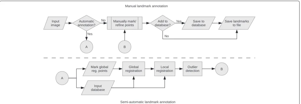
The automatic landmark annotation process was based on a hierarchical, free-form registration of image patches from the database to the query image. The sequence of processes involved is shown in Figure 1. An initial align-ment was derived from four landmark points, by min-imising the root-mean-squared (RMS) distances between corresponding points over a nine-parameter affine trans-formation (i.e. 3D translation, rotation and scale) using the simplex algorithm [47]. Figure 2 shows a typical image volume for experiments in landmark-base
geo-metric morphogeo-metrics, a 3D micro-CT image of aMus
musculus specimen, together with manual annotations of a typical set of landmarks, described in detail in Table 1. Four typical global registration points are shown in Figure 2b. An automated check was implemented to ensure that the points were not coplanar. This point-based registration could have been decomposed into individ-ual transformations, deriving the translation parameters by aligning the centroids of the four points and the scal-ing parameters from the standard deviations of the points, leaving only the rotation to be obtained through optimi-sation. However, in practice all nine parameters of the transformation model were obtained via the optimisa-tion, so that the distance between the centroids of the points in each registered image volume could be used as a semi-independent, automated check.
Once the initial manual alignment had been obtained, it was used to initialise a multi-stage automatic registra-tion process. The first stage was performed on the entire image volume, and optimised a nine-parameter affine transformation using the simplex algorithm [47]. The lat-ter stages operated on patches of image data around each landmark point. As described above, the intention was to terminate the process with patches small enough that the effects of shape variation between the database and query images were minimised. However, registration of small patches had a correspondingly small capture range: in preliminary work, a single stage of patch-based registra-tion proved to be insufficient to attain accuracies equiv-alent to manual annotation. Therefore, additional stages of patch-based registration were included, with the patch size reduced between each stage; an empirical evaluation of accuracy and time versus the number of registration stages was performed, and the optimal number of patch-based stages was shown to be three, for a total of five stages of registration including the point-based initiali-sation and the global, image-based stage (see Additional file 1). Some experiments in geometric morphometrics
(a) (b)
(c)
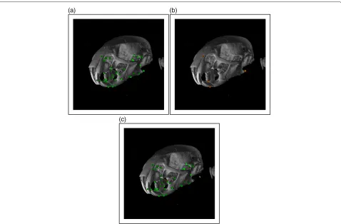
Figure 23D renderings of the automatic landmark point annotation process on aMus musculusspecimen.(a)Manual annotation of the 40 mandible landmarks.(b)Four of the manual landmarks used in the global registration.(c)Automatically annotated landmarks, derived using a database of sevenMusspecimens. Landmarks passing the outlier test are shown in green: those failing are shown in chequered green and red.
may include landmarks specified as the extremal points on curved surfaces from certain view directions. The inclu-sion of rotation in the patch-based registration would destabilise the registration in such cases (e.g. registra-tion of an arc of a circle to that circle is degenerate over rotation, but not translation or scaling). Therefore, the transformation model used in the patch-based stages of registration consisted only of 3D translation and scal-ing. Each stage of registration was initialised using the concatenation of the transformation matrices from all pre-vious stages. However, a simple check was included to prevent problems with fit failures; if the result after any stage of registration generated a projected location that lay outside the boundaries of the query image volume, then the parameters of that stage were set to an identity transformation.
Since a nine-parameter affine transformation model was used, the problem was over-determined with realistic patch sizes. Therefore, rather than using cuboids from the data as image patches, 2D slices aligned to the major axes of the image volume and centred on the landmark points were used; in the first stage, operating on the entire image volumes, the slices were taken through the centre points
of the volumes. This considerably reduced the amount of data included in the cost function calculation, and so reduced the processor time required whilst still achieving sufficient levels of accuracy.
The cost function for all automatic registration stages was theχ2per degree of freedom of the scaled images or image patches (a derivation is provided in Appendix A)
χ2= 1
(N−D)
v
(Jv−γIv)2
σ2
J +σI2γ2
where γ = |J| |I| (1)
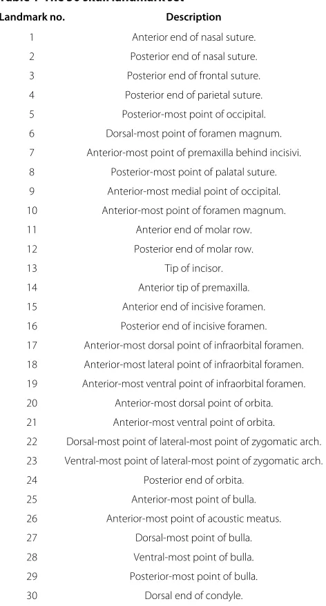
Table 1 The 50 skull landmark set
Landmark no. Description
1 Anterior end of nasal suture.
2 Posterior end of nasal suture.
3 Posterior end of frontal suture.
4 Posterior end of parietal suture.
5 Posterior-most point of occipital.
6 Dorsal-most point of foramen magnum.
7 Anterior-most point of premaxilla behind incisivi.
8 Posterior-most point of palatal suture.
9 Anterior-most medial point of occipital.
10 Anterior-most point of foramen magnum.
11 Anterior end of molar row.
12 Posterior end of molar row.
13 Tip of incisor.
14 Anterior tip of premaxilla.
15 Anterior end of incisive foramen.
16 Posterior end of incisive foramen.
17 Anterior-most dorsal point of infraorbital foramen.
18 Anterior-most lateral point of infraorbital foramen.
19 Anterior-most ventral point of infraorbital foramen.
20 Anterior-most dorsal point of orbita.
21 Anterior-most ventral point of orbita.
22 Dorsal-most point of lateral-most point of zygomatic arch.
23 Ventral-most point of lateral-most point of zygomatic arch.
24 Posterior end of orbita.
25 Anterior-most point of bulla.
26 Anterior-most point of acoustic meatus.
27 Dorsal-most point of bulla.
28 Ventral-most point of bulla.
29 Posterior-most point of bulla.
30 Dorsal end of condyle.
These landmarks were identified on the 12-element data set described in Table 4. Points 11 to 30 were identified on the left-hand-side of the specimen; points 31 to 50 were the equivalent points on the right-hand side of the specimen.
parameters and average bone density. Trilinear interpola-tion was used in the resampling. The scaling factor was obtained through a maximum-likelihood based approach (see Appendix A). Inevitably, the scaling could be puted only from aligned images. Therefore, it was com-puted after the point-based stage of registration, and then remained fixed through all of the image-based registra-tion stages. Preliminary work on this topic was described in [48].
In order to reduce the noise on the images and thus pro-vide a smoother cost function, reducing the probability that the optimisation would become trapped in a local
minimum, Gaussian smoothing was applied to all image patches prior to registration. The kernel was truncated at three standard deviations from the mean and, in order to ensure that no edge effects were present, a boundary region equal to three standard deviations of the smooth-ing kernel was added around all stored image patches and included in the smoothing, but excluded from the
χ2 calculation, thus ensuring that all smoothed
vox-els contributing to the χ2 were calculated from equal numbers of un-smoothed voxels and avoiding truncation effects.
Rather than operating directly on the image intensities, the cost function was applied to image intensity gradients in order to provide further robustness to differences in average bone density or scanner parameters. This strategy has been found useful in other applications that require matching of similar but non-identical images e.g. stereo pairs of natural scenes [49]. Images showing the gradient components in thexandydirections of each patch were calculated, for each of the three orthogonal patches pass-ing through each landmark point, uspass-ing finite differencpass-ing i.e. taking the intensity difference between neighbouring voxels in the relevant direction. This gave a total of six gradient patches for each landmark. The cost function was applied to each gradient patch separately and the results summed to produce a singleχ2per degree of free-dom. Note thatNin Eq. 1 refers to the total number of voxels included in the three orthogonal patches, not the total number in the six gradient patches, since thex- and y-gradients of each patch were obtained from the same original data.
Explicit inclusion of the noise term in the cost function allowed theχ2 per degree of freedom at the end of the registration to be used as a check on registration error, through comparison to theχ2distribution. The noise on the original images was estimated from the width of zero crossings in horizontal and vertical gradient histograms [50]. Smoothing reduced the noise by a factor of 4πσK2 where σK was the standard deviation of the smoothing kernel [51] (see Appendix B). The calculation of image gradients by finite differencing introduced a further factor of√2 into the noise calculation.
J image voxel was zero padded; the fourth combination, where both voxels were zero-padded, was identically zero. The correct noise term was used in each case (σJ2+γ2σI2,
γ2σ2
I, andσJ2respectively, divided by the correction fac-tors for smoothing and differentiation). These threeχ2 terms were then summed prior to division by the number of degrees of freedom, the total number of voxels included in all three terms minus the number of parameters in the transformation model.
Array-based voting
The result from the various stages of registration was a projected location, in the coordinate system of the query image, for each landmark point in each database entry. These constituted multiple estimates of the position of each landmark in the query image, with the number of estimates equal to the number of database entries. The multiple estimates for each landmark were then combined in order to generate a single, final estimate of the loca-tion of that landmark in the query image. However, it could not be guaranteed that all estimates were accurate; if one of the database images exhibited significant shape difference, compared to the query image, in the region around one of the landmark points, then it would pro-vide a poor model for that landmark. The corresponding registration would then be likely to fail, resulting in an out-lier amongst the multiple estimates for the landmark. Any simple method of combination, such as taking the mean of all estimates, would be affected by the presence of such outliers.
Instead, a method that was robust to outliers was imple-mented, based on the array-based voting used in methods such as the Hough transform; the same approach has proven reliable in shape-model based approaches to the annotation of landmark points on both clinical and non-clinical images (e.g. [45,52,53]). The voting method was applied to each landmark independently. The multiple estimates for the position of a landmark were analysed to find the maximum and minimum values of theirx,yand zcoordinates; this specified a 3D volume large enough to contain the estimates. An array of this size was created, and a value of unity was entered into the array at the posi-tion of each estimate. The array was then smoothed using a Gaussian kernel, approximating the random error on the registration results. The kernel size was a free param-eter of the algorithm (see Additional file 1 and see the Conclusions for further comments). Assuming that the majority of the database images provided good models of the query image, the entries in the voting array would include a compact distribution located close to the correct position for the landmark, representing successful regis-trations. The width of this distribution would be dictated by the random error on the registration, which would in
turn be dictated by the noise on the original images. In contrast, outliers would by definition be scattered far from the correct position. Therefore, smoothing the array with a kernel corresponding to the random error on success-ful registrations would result in a single, main peak at the position of the compact group of accurate estimates, and a number of smaller, secondary peaks at the positions of outliers. The position of the highest peak in the smoothed array was taken as the final estimate of the landmark location, producing a method that combined the multiple estimates of each landmark location whilst being robust to the presence of outliers.
Prior to creation of the voting array for each land-mark point, the projected locations of the corresponding database points in the coordinate system of the query image were compared to the boundaries of that image; any point lying outside the boundary plus a border of three times the standard deviation of the smoothing kernel was omitted from the voting process, in order to prevent prob-lems with severe outliers, on the basis that these points could not contribute to a valid final estimate in any case. The size of the array was then determined by finding the range of the projected locations for the remaining points.
Outlier detection
In order for the final algorithm to have any utility, it was essential that it should provide a reliable indica-tion of the accuracy of automatic annotaindica-tions; otherwise, much of the manual interaction that it was intended to replace would be re-introduced through a requirement for manual inspection of the results. The array-based vot-ing described in the previous section required that the majority of the multiple estimates of the position of each landmark were located close to the correct position; if this were not the case, due to significant differences in shape between the query image and all of the database images, then the voting would produce an incorrect result. An out-lier detection method with an extremely low false positive rate, i.e. an extremely low number of outliers flagged as accurate annotations, was therefore required.
distribution, i.e. the multiple estimated landmark loca-tions generated from the database images will be ran-domly scattered around the true landmark location in the query image according to a distribution dependent on random shape differences (which could be termed “shape noise”). This will add to the distribution due to random image noise, and so the MVB will provide an underesti-mate of the true distribution of the estiunderesti-mated landmark locations.
As stated above, [28] and [29] developed a method that measured the shape of the cost function around the optimum using the eigenvectors of the Hessian matrix, allowing the rejection of results where shape differences destabilised the registration to the point where there was no clear optimum. However, this method was limited to analysis of the cost functions for individual registra-tions. In the work described here, the multiple registration results for each landmark supported an analysis of the distribution of registration parameters induced by shape variation between the database images. The number of samples available was too small to allow a full charac-terisation of the distribution; therefore, unreliable results were identified through an analysis of the available point estimates. The individual registration results were first sorted into order based on theχ2per degree of freedom at the end of the registration process. The distances between the results and the final location generated by the array-based voting were then compared to a threshold, treating each distance as an estimate of the standard deviation of the distribution. The threshold and the number of com-parisons performed were free parameters of the algorithm (see Additional file 1); in practice, comparison to three points proved optimal. Any final location for which any one of the three registration results with the lowestχ2per degree of freedom was more distant than the threshold was flagged as a potential outlier. The technique there-fore imposed a requirement that the patches which were estimated to provide the best models of the query image patch, based on theirχ2per degree of freedom, formed a distribution within the voting array no broader than the threshold.
Software
The semi-automatic landmark point localisation algo-rithm was implemented within the TINA Geometric Morphometrics toolkit, which also includes the TINA Manual Landmarking tool [8], and algorithms that per-form quantitative shape analysis with weighted covari-ance estimates for increased statistical efficiency [54]. This package has been made available as free and open source software (FOSS) under the GNU General Public Licence (www.gnu.org), and can be obtained via the TINA web-site (www.tina-vision.net). The User Manuals for the TINA Geometric Morphometrics toolkit and the TINA
software are included Additional files 2 and 3, respec-tively. Figure 1 shows the sequence of operations involved in semi-automatic landmarking, and how the algorithm interfaces with the manual annotation software. Figure 3 shows a screen-shot of the software in operation. The 3D renderings and associated landmark annotations are shown in more detail in Figure 2.
Results and discussion
Evaluation of the algorithm was performed using micro-CT images of rodent skulls with an in-plane resolution of 635×635 voxels and between 1000 and 1500 slices, with voxel dimensions of 0.035 mm along all axes. A detailed description of all image volumes and landmark points used is provided in Tables 1, 2, 3 and 4. The algorithm included a number of free parameters, such as image patch and smoothing kernel sizes for each stage of reg-istration. As described in Additional file 1, these were optimised using a data set of 8Musspecimens of varying species (see Table 2) with expert manual annotation of 40 mandible landmarks (see Table 3). All manual annotations were performed using the TINA software [8].
In order to avoid any bias, the evaluation of automatic point localisation accuracy was performed on a data set of 12 Mus musculus specimens from consomic strains, independent of those used in the parameter optimisa-tion experiments (see Table 4). Two sets of expert manual annotations of 50 skull landmarks were performed on each (see Table 1), allowing estimation of manual anno-tation repeatability; the repeat annoanno-tation was performed after an interval of one week, in order to minimise bias due to training effects. Separate experiments were performed for each set of manual annotations in sets of leave-one-out experiments, using 11 specimens to construct the training database and the 12th as the query image, repeat-ing for all 12 image volumes. Four manually annotated points in each volume were used to provide the initial, global alignment; however, the locations of these points were re-estimated by the automatic annotation algorithm, such that results were not contaminated with manual annotations.
Figure 3Screen-shot of the semi-automatic landmark annotation software.
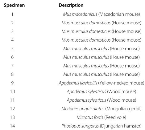
Table 2 The 8- and 14-element data sets
Specimen Description
1 Mus macedonicus(Macedonian mouse)
2 Mus musculus domesticus(House mouse)
3 Mus musculus domesticus(House mouse)
4 Mus musculus domesticus(House mouse)
5 Mus musculus musculus(House mouse)
6 Mus musculus musculus(House mouse)
7 Mus musculus musculus(House mouse)
8 Mus musculus musculus(House mouse)
9 Apodemus flavicollis(Yellow-necked mouse)
10 Apodemus sylvaticus(Wood mouse)
11 Apodemus sylvaticus(Wood mouse)
12 Meriones unguiculatus(Mongolian gerbil)
13 Microtus fortis(Reed vole)
14 Phodopus sungorus(Djungarian hamster)
The 8-element data set consisted of the first 8 specimens, all of which were various species from the genusMus. The 14-element data set also included specimens from other genera. Expert manual annotation of 40 mandible landmarks was performed for each specimen; see Table 3 for details.
from the corrected landmarks. However, the number of such errors, 4% of the points in the first set of manual landmarks and 0.5% of the points in the second set, was recorded, and the lower value used as a target for the false positive rate of the error detection stage of the automatic point localisation algorithm.
In order to calculate true and false positive and nega-tive rates for the outlier test, a threshold value on point localisation error in voxels was required. This is referred to in the following sections as the error threshold, and was determined using the repeatability of the manual
annotations on the 12 consomic Mus musculus
Table 3 The 40 mandible landmark set
Landmark no. Description
1 Tip of incisor.
2 Dorsal-most point of incisive alveole.
3 Ventral-most point of diastema.
4 Anterior-most point of molar row.
5 Posterior-most point of molar row.
6 Lateral point of mandibular foramen.
7 Tip of coronoid process.
8 Anterior-most point of curve between coronoid and articular process.
9 Ventral-most point of curve between coronoid and articular process.
10 Anterior-most point of condyle.
11 Lateral-most point of condyle.
12 Posterior-most point of condyle.
13 Anterior-most point of curve between articular and angular process.
14 Tip of angular process.
15 Medial-most point of angular process.
16 Lateral point of masseteric crista at dorsal-most ventral point.
17 Lateral-most inner point of ventral border.
18 Anterior end of attachment area of transverse mandibular muscle.
19 Posterior-most point of incisive alveole.
20 Anterior end of masseteric crista.
These landmarks were identified on the 8- and 14-element data sets described in Table 2. Landmarks 1–20 consisted of these points on the left-hand side of the specimen; landmarks 21–40 consisted of the same points on the right-hand side of the specimen.
Figure 4 shows the results of the leave-one-out exper-iments performed on the data set of 12 image volumes of consomicMus musculus specimens using the second set of manual landmarks to produce the database and using four manual annotations to perform the initial, manual stage of alignment. The results are presented as box-and-whisker plots of the Euclidean distance in voxels between the automatic and manual annotations for each point, showing the median, minimum, maximum, 25th and 75th percentiles. The ROC curve, generated by vary-ing the outlier test threshold, shows that the threshold and number of points included, derived from an indepen-dent data set, were approximately optimal for these data; there were no false positives at the operating point used, i.e. all 525 points passing the test were within the error threshold of 30 voxels. Across all twelve volumes, 87.5% of the automatic annotations passed the outlier test, and 98.3% were within the error threshold. In a hypothetical annotation process with a pre-built database, this level of
Table 4 The consomicMus musculusspecimens included in
the 12-element data set
Specimen Description
1 PWD/Ph (wild-derivedMus musculus musculusstrain)
2 PWD/Ph (wild-derivedMus musculus musculusstrain)
3 PWD/Ph (wild-derivedMus musculus musculusstrain)
4 PWD/Ph (wild-derivedMus musculus musculusstrain)
5 C57BL/6J-10dPWD/Ph
6 C57BL/6J-10dPWD/Ph
7 C57BL/6J-7PWD/Ph
8 C57BL/6J-7PWD/Ph
9 C57BL/6J-7PWD/Ph
10 C57BL/6J (Mus musculus domesticusbackground)
11 C57BL/6J (Mus musculus domesticusbackground)
12 C57BL/6J (Mus musculus domesticusbackground)
This data set included several specimens of each pure strain (C57BL/6J and PWD/Ph), together with specimens in which chromosomes 7 or 10 from theMus
musculus musculusstrain PWD/Ph had been substituted into theMus musculus
domesticusstrain C57BL/6J. Expert manual annotation of 50 skull landmarks was
performed for each specimen; see Table 1 for details.
performance equates to a potential user of the software having to manually inspect 12.5% of the points, but having to correct the positions of fewer than 2% of the points, i.e. fewer than 12 points. Therefore, combined with the four points per specimen required for the initial, point-based stage of registration, the user would be required to man-ually annotate an average of 5 points per specimen out of a total of 50 landmark points i.e. one tenth of the total number of points.
1 2 3 4 5 6 7 8 9 10 11 12 Sample
10 20 30 40 50
P
oint Error (v
o
x
els)
0 20 40 60 80 100
Points
passing
outlier
test
(
%
)
(a)
0.2 0.4 0.6 0.8 1 1.2 1.4 False Positive ( %)
20 40 60 80 100
True Positive (%)
(b)
Figure 4Automatic landmark annotation accuracy using an initial, point-based registration.(a)Box-and-whisker plots of the point localisation errors for automatic annotation of 50 skull landmarks on the 12 consomicMus musculusspecimens (read against the left-hand scale), using the second set of manual landmarks and an initial, point-based registration stage. The black squares and red crosses show, respectively, the percentage of points passing the outlier test and the percentage within the error threshold (read against the right-hand scale); only points passing the outlier test have been included in the box-and-whisker plots.(b)ROC curve of the true and false positive rates of points passing the outlier test; the operating point of the test is coincident with the y-axis.
again assuming equal errors on the two sets of results, the median of the automatic annotation error on a sin-gle point was approximately 1.0 voxels. The mean of the worst outliers in all twelve volumes was 7.4 voxels. Only automatically located points passing the outlier test were included in the results; this was 81.8% of the points across all 12 volumes. Due to the non-Gaussian distribution of the annotation errors, the manual and automatic repeata-bilities were compared using a Mann-Whitney U test,
which conclusively demonstrated (U = 72116, Uμ =
147300, Uσ = 5187, Z = −14.52, p ≈ 0) that the
automatic repeatability was significantly better than the manual repeatability.
Evaluating the repeatability of the automatic annota-tion did not evaluate its accuracy; such an evaluaannota-tion was not possible without a set of gold-standard (i.e. error-free) landmark locations. However, comparison of the median Euclidean distance in voxels between the two sets of man-ual annotations (3.34 voxels) and the median Euclidean distance between the second set of manual annotations and the automatic annotations derived from them (3.6 voxels) indicated no statistically significant difference
(Mann-WhitneyU =149405,Uμ=157200,Uσ =5429, Z = −1.44, p = 0.15). This indicated that automatic annotation was not significantly less accurate than manual annotation.
Double iteration without point-based registration
The reliability of the outlier test, demonstrated in the experiments described above, allows an alternative mode of operation for the algorithm that can potentially elim-inate the need for manual annotation of the four points used in the initial stage of global registration. The gross misalignments between image volumes, for which this stage of registration was designed, can be avoided if care is taken during the preparation of specimens, such that they are all scanned in approximately the same orientation. The algorithm can then be applied in two stages; a first pass, with no point-based registration, generates an inter-mediate set of automatic annotations. Fewer points will pass the outlier test; however, the points that do can be used to perform the point-based stage of registration in a second pass of the algorithm. A second set of experi-ments, identical to those described above but using this
1 2 3 4 5 6 7 8 9 10 11 12 Sample
10 20 30 40 50
Point Error
(voxels
)
(a)
1 2 3 4 5 6 7 8 9 10 11 12 Sample
10 20 30 40 50
Point Error
(voxels
)
0 20 40 60 80 100
Points passing outlier test
(%
)
(b)
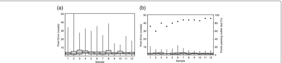
“double-pass” mode of operation, was performed in order to test this approach. The results for automatic annota-tion using a database built from the second set of manual annotations are shown in Figure 6. The median Euclidean distance between the manual and automatic annotations across all twelve volumes was 3.49 voxels, compared to 3.60 voxels for the equivalent experiment in single-pass mode, but the difference was not statistically significant (Mann-WhitneyU=134236,Uμ=137550,Uσ =4906, Z = −0.68,p = 0.50). Similarly, there was no signifi-cant difference between the number of points passing the outlier test (87.5% in single-pass and 87.3% in double-pass mode) or the percentage of points with errors lower than the error threshold (98.3% in single-pass and 97.8% in double-pass mode). The ROC curve shows that the out-lier test parameters, derived from an independent data set, were approximately optimal for these data; the false positive rate of the outlier test was 0.17%, i.e. across the 600 points in the 12 volumes, i.e. only one point with an error larger than the threshold was not flagged as an outlier. Figure 7 shows a comparison of the repeatabil-ity of manual and automatic landmark annotation when the software was used in double-pass mode; as with the single-pass mode, the automatic repeatability was signifi-cantly better (Mann-WhitneyU =77551,Uμ =146700, Uσ = 5162,Z = −13.39, p ≈ 0). However, it should be noted that the double-pass mode of the algorithm is dependent on the alignment of the specimens within the scanner, and is likely to fail if significant misalignments are present.
Multiple-genera database
In order to evaluate the robustness of the algorithm to databases containing specimens with significant shape differences, a further data set consisting of 14 micro-CT image volumes of rodent skulls from multiple gen-era was used (see Table 2), with manual annotations
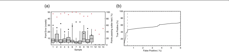
of 40 mandible landmarks on each (see Table 3). This was a superset of the 8 Mus skull data set used in the parameter optimisation experiments, and was therefore not completely independent (i.e. the free parameters of the algorithm were partially derived from this data set), although the evaluation of the free parameters showed a high degree of independence between performance and parameter values (see Additional file 1 for details). In addi-tion to the 8Mus specimens, the data set included one Apodemus flavicollis, twoApodemus sylvaticus, one Meri-ones unguiculatus, oneMicrotus fortisand onePhodopus sungorusspecimen. This combination of specimens was chosen to exhibit a range of shape variation, i.e. the Apode-musspecimens were more similar in shape to the Mus specimens than were the Microtus, Phodopus or Meri-onesspecimens. The skull constituted the majority of the bone surfaces in the images and so dominated the regis-tration result; the mandible is not rigidly fixed to the skull, and so the use of mandible landmarks provided a more significant challenge to the algorithm and was more suit-able to illustrate failure modes. As above, the automatic point localisation algorithm was applied to the data in a set of leave-one-out experiments, using 13 image volumes to construct the database and predict landmark locations in the 14th volume, repeating for all 14 volumes. A sec-ond set of experiments was csec-onducted using only the eight Musspecimens from the data set. The results are shown in Figures 8 and 9.
The effects of building the database from multiple gen-era can clearly be seen in the breakdown of the results by genus. During annotation of theMicrotus,Phodopus and Meriones specimens, which varied significantly in shape from theMusandApodemusspecimens, there were no similar specimens in the database and consequently the outlier test rejected all points. The median landmark error across theMusspecimens was slightly lower using a mixed-genera database than using aMus-only database
1 2 3 4 5 6 7 8 9 10 11 12 Sample
10 20 30 40 50
Point Error (voxels)
0 20 40 60 80 100
Points
passing
outlier
test
(
%
)
(a)
0.25 0.5 0.75 1 1.25 1.5 1.75 2 False Positive ( %)
20 40 60 80 100
True Positive (%)
(b)
1 2 3 4 5 6 7 8 9 10 11 12 Sample
10 20 30 40 50
Point Error (voxels)
(a)
1 2 3 4 5 6 7 8 9 10 11 12 Sample
10 20 30 40 50
Point Error (voxels)
0 20 40 60 80 100
Points
passing
outlier
test
(
%
)
(b)
Figure 7Repeatability of manual and “double-pass” automatic landmark annotation.Box-and-whisker plots of the repeatability of manual(a) and automatic(b)(read against the left-hand scale) localisation of 50 skull landmarks on the 12 consomicMus musculusspecimens. The automatic landmarks were generated using the “double-pass” mode with no initial, point-based stage of global registration. Only points passing the outlier test were included in the automatic annotation results; the black squares show the percentage of points passing (read against the right-hand scale).
(5.11 voxels compared to 5.24 voxels); however, the dif-ference was not statistically significant (Mann-Whitney U = 21464,Uμ = 21830,Uσ = 1239,Z = −0.30,p = 0.77), indicating that the additional specimens added little information. However, their presence did lead to a marked reduction in the number of points passing the outlier test (57.8% compared to 73.8%), although the percentage of points with errors lower than the error threshold was not significantly different (95.0% vs. 95.3%). The median annotation errors on theApodemusspecimens were larger than those on the Mus specimens (6.83 voxels vs. 5.11 voxels), but the difference was on the borderline of statis-tical significance (Mann-WhitneyU =4545,Uμ=5428, Uσ =506,Z= −1.75,p=0.08).
These results serve to indicate the robustness of the algorithm to variations in the database. When specimens from multiple genera with significant variation in shape were entered into the database, only those with simi-lar shape to the query image contributed information to the final landmark location estimate. Conversely, for those specimens where the database provided no usable information, the algorithm successfully indicated that the automatic annotation was not reliable and rejected all
points. Contamination of the database with multiple gen-era did not result in a significant decrease in landmark annotation accuracy, but did result in a large reduction in the number of points passing the outlier test, reflect-ing the bias of the outlier test towards low false positive rates.
Database size and processor time requirements
The dependence of algorithmic performance on the num-ber of image volumes in the database was evaluated by repeating the leave-one-out experiments on the 12 consomicMus musculusspecimens with fewer database entries. In order to avoid confounding the results by vary-ing several features of the experimental procedure simul-taneously, databases with fewer than three entries (the smallest number required to perform the outlier test) were not considered, and the image volumes included were selected randomly. The results are shown in Figure 10; each box-and-whisker shows the point localisation errors in voxels across all 12 volumes. Only points passing the outlier test were included, and the percentage of such points is also shown. The results demonstrate that, as would be expected, the point localisation errors decreased
1 2 3 4 5 6 7 8 9 10 11 12 13 14 Sample
10 20 30 40 50
Point Error (voxels)
0 20 40 60 80 100
Points
passing
outlier
test
(
%
)
(a)
1 2 3 4 5 6
False Positive ( %) 20
40 60 80 100
True Positive (%)
(b)
1 2 3 4 5 6 7 8 Sample
10 20 30 40 50
Point Error (voxels)
0 20 40 60 80 100
Points
passing
outlier
test
(
%
)
(a)
1 2 3 4 5
False Positive ( %) 20
40 60 80 100
True Positive (%)
(b)
Figure 9Automatic landmark annotation accuracy using 8Musspecimens from the mixed-genera database.(a)Box-and-whisker plots of the point localisation errors for automatic annotation of 40 mandible landmarks on the data set of 8Musspecimens (read against the left-hand scale). The black squares and red crosses show, respectively, the percentage of points passing the outlier test and the percentage within the error threshold (read against the right-hand scale); only points passing the outlier test have been included in the box-and-whisker plots.(b)ROC curve of the true and false positive rates of points passing the outlier test; the dashed line shows the operating point.
with increasing database size and the number of points passing the outlier test increased. However, both depen-dencies were relatively weak with this data set; there was little improvement in performance with database sizes larger than eight entries. This is significantly fewer images than would be required for the construction of an appear-ance model.
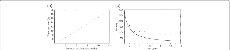
The processor time requirements of the algorithm were also evaluated during the tests on database depth. Exper-iments were performed on a Dell Precision worksta-tion with 2 Intel Xeon 5670 processors and 24 Gb of main memory, running OpenSuse 11.3×64 (Linux kernel 2.6.34). It was anticipated that, in practical use, a single database would be constructed and then used to anno-tate multiple image volumes. Therefore, the database and image loading times were ignored and the wall-clock time required to perform the registration, array-based voting and outlier test was measured. Figure 11 shows the results, averaged over all experiments performed at each database size, as the number of seconds required to annotate a single point. The vast majority of the time taken to run the algorithm was accounted for by the registrations and so, since the registrations were per-formed independently for each database entry, there was
a linear dependence on the number of entries. The gra-dient of the linear fit, i.e. the time taken per point per database entry, was 1.64 seconds. In [8], the time required to manually annotate 10 landmarks on the mandible in micro-CT images of three rodent specimens (Microtus, MusandPachyuromys) was evaluated in both TINA and AMIRA (www.vsg3d.com/amira), both by a non-expert and an expert AMIRA user. Average timings were 13s per point using AMIRA and 30s per point using TINA for the expert, and 54s per point using AMIRA and 65s per point using TINA for the non-expert, although strong training effects were observed with TINA, as would be expected of users handling unfamiliar soft-ware. Therefore, assuming a reasonable database size of around 8 entries and thus approximately 13s per point for automatic annotation, the time required to per-form automatic annotation was comparable to the time required to perform manual annotation with AMIRA. However, unlike manual annotation with AMIRA, auto-matic annotation with TINA does not require continu-ous user input. Comparison between TINA and AMIRA in terms of manual annotation accuracy is provided by [8]; note that AMIRA does not provide automatic annotation.
3 4 5 6 7 8 9 10 11 Number of database entries 10
20 30 40
Point Error (voxels)
0 20 40 60 80 100
Points
passing
outlier
test
(
%
)
(a)
3 4 5 6 7 8 9 10 11 Number of database entries 2
4 6 8 10
Point Error (voxels)
0 20 40 60 80 100
Points
passing
outlier
test
(
%
)
(b)
4 6 8 10 12 Number of database entries 6
8 10 12 14 16 18 20
Time per point (s)
(a)
2 4 6 8 10 12 No. Cores
500 1000 1500 2000 2500 3000
Time (s)
(b)
Figure 11Dependence of run time on database size and the number of cores in use.(a)The average wall-clock time required to perform all registration stages, array-based voting and the outlier test on the 50 skull landmarks in each of the 12 consomicMus musculusspecimens, plotted against the number of image volumes in the database. The dashed line shows a linear fit to the data.(b)The average wall-clock time required to perform all registration stages, array-based voting and outlier test on 50 skull landmarks in each of the the 12 consomicMus musculusspecimens with 11 database entries, plotted against the number of processor cores used. The 1/cores curve that would be achieved with 100% parallelisation efficiency is also shown.
The software made extensive use of parallelisation, and so the dependence of the run time on the number of pro-cessor cores in use was also evaluated. Figure 11 shows the time taken to perform the registration, array-based voting and outlier test stages of the algorithm in leave-one-out tests on the 12 consomic Mus musculus speci-mens (i.e. with a database size of 11), averaged over the 12 experiments, against the number of processor cores, together with the 1/cores dependency that would be expected if the parallelisation efficiency was 100%. The results showed good parallelisation efficiency up to three cores, little further reduction in the time taken until six cores were in use (allowing full parallelisation over the six image patches for each landmark point; see the Methods section for details), and then no further reduction. The loss of parallelisation efficiency above three cores indi-cates that memory bandwidth was the main limiting fac-tor, due to the algorithm performing large numbers of relatively simple operations on small blocks of data. How-ever, these results indicate that the timings described above should be achievable on most relatively modern hardware.
Conclusions
Geometric morphometric analyses, consisting of manual annotations of landmark points followed by Procrustes analysis, are a popular way to quantify biological shapes for comparison to genetic, phylogenetic or ecological fac-tors. The requirement for extensive and time-consuming manual annotation places practical limitations on the number of specimens that can be included in such analy-ses, in turn limiting their statistical power both in terms of the magnitude of shape variation that can be measured and the confidence intervals on any conclusions. In this paper, a semi-automatic landmark annotation algorithm designed to accelerate the landmark annotation process has been presented.
The aim was to produce landmarks for use in shape analysis, and so no constraint based on a shape model, or assumptions about shape, could be used in the algo-rithm. These models or assumptions would be recovered by the subsequent analysis and therefore potentially bias the results if they were not a perfect fit to the data. Instead, a free-form, intensity-based registration approach was adopted. Multiple example images, each with manually annotated landmarks, were registered to the query image using a multi-scale approach. The final stages of regis-tration operated on small patches of image data around each landmark in order to minimise the effects of global shape variation. This resulted in one set of estimated landmark locations for each database image; these were combined using a Hough-like voting array in order to introduce robustness to biases and outliers whilst min-imising assumptions about their distribution.
model of the query image, and used a minimal assump-tion that good models should produce a compact peak in the Hough-like voting array, whilst poorly fitting models should produce a broad outlier distribution.
In order to have utility within the target user commu-nity, the algorithm had to perform landmark annotation as quickly and as accurately as manual annotation; therefore, evaluation focused on these two properties. Comparisons were performed between two independent sets of man-ual annotations of 50 skull landmarks in 12Mus musculus specimens, and two sets of automatic annotations gen-erated from them. Automatically annotated points failing the outlier test were not included in the comparisons. For the 87.5% of the points that were included, the results showed that automatic annotation was at least as accu-rate as, and more repeatable than, manual annotation, i.e. had a lower random error and no significant systematic error. The repeatability of the automatic annotations indi-cated that voxel-level accuracy was achieved. The outlier test proved extremely reliable, rejecting 12.5% of the auto-matic annotations to achieve a false positive rate of less than 0.5%, due to the care taken in the estimation of noise distributions.
The evaluation on a wider variety of rodent specimens, including multiple genera, demonstrated the reliability of the outlier test. In cases where the database contained no specimen that provided a good model of the query image, the algorithm correctly flagged all points as outliers. Con-versely, the presence of database specimens that provided poor models of the query image did not significantly affect the accuracy of the automatic annotation process, even where they formed the majority of the database. This sug-gests an iterative mode of operation; any query image that generates large numbers of outliers is not well modelled by the existing database. Therefore, after manual correction of the outliers, it can be added to the database in order to expand the number of specimens that can be annotated accurately.
Timing tests demonstrated that the automatic land-mark localisation process required approximately the same wall-clock time as manual annotation on reasonably modern hardware. However, no user input was required for this stage of the process. Therefore, actual manual annotation required for each image volume in a hypo-thetical landmark annotation process would be limited to the four registration points, visual check of the detected outliers, the majority of which would be in the correct location due to the low false-positive bias of the out-lier detector, and correction of the true outout-liers, which averaged around 1 to 2 points per volume with a single-genera image database. For realistic landmark list sizes of 40 to 50 points, the automatic landmark localisation software could therefore reduce the required number of manual landmark annotations by a factor of ten. Further
improvements were achieved using the double-pass mode of operation, although this would require care during sam-ple preparation to ensure a reasonably good alignment of the samples within the image volumes. Annotation of the training images constitutes the majority of the manual annotation required when using the proposed technique. However, the evaluation of database size in the
experi-ments on consomic Mus musculusspecimens indicated
that only eight images were required, far fewer than would be required by alternative techniques based on statistical shape models.
Several potential routes exist for future improvement of the software. For instance, it may be possible to automat-ically estimate patch sizes using techniques such as those described in [12], reducing the need to optimise the free parameters of the algorithm prior to application to new image types. Furthermore, annotation of the four points used to initialise the global registration requires signifi-cant user interaction. This could be simplified using the 3D rendering of the data provided by the software, by prompting the user to rotate the rendering into a standard orientation, which would then provide the initialisation. A similar orientation would have to be stored for each of the images in the database.
The software described in this paper has been made available as free and open source (FOSS) software under the GNU General Public Licence (www.gnu.org), and can be obtained via our web-site (www.tina-vision.net).
Appendix A: derivation of the cost function and scaling factor
Let Iv and Jv be corresponding voxels in two identical, noise-free images or image patches I and J. Scale the intensities of one of the images by a factorγ; without loss of generality, assume that this is imageJ. Add Gaussian random noise with standard deviations ofσIandσJto the two images. Find an estimator forγ.
The derivation given here follows that given in [55]. An estimator ofγ can be obtained as the gradient of a linear fit toJvvs.Ivover allvwith an intercept of zero, as shown in Figure 12. Since there is noise on bothIandJ, the noise-free intensities of a pointA = Iv,Jvcould correspond to any pointCalong the linear fit. However, ifσI = σJ = σ, the probability that a datum atAwas generated fromCis given by
P(C→A) = 1 2πσ2exp
−(IC−IA)2 2σ2
exp
−(JC−JA)2 2σ2
= 1
2πσ2exp
− r2
2σ2
= 1
2πσ2exp
− h2
2σ2
exp
− u2
2σ2
A
B
C
D
I J
u r
h
Figure 12The construction of theχ2between two scaled image
patches.A linear fit to the joint intensity histogram of a pair of imagesIandJ. Since both images contain noise, a datum at point A could be generated from any point C along the linear fit. However, if the standard deviations of the noise onIandJare equal, then the probability of generating data at A depends only on the perpendicular distancehto the linear fit, not onu.
Integrating overu gives a constant σ√2π, so the prob-ability depends only onhi.e. only on the perpendicular distance to the line. In the event thatσI =σJ, the images can be scaled toI=I/σIandJ=J/σJ.
The distancehcan be obtained from the vectors A =
(Iv,Jv)andB=(Iv,γIv)using
A.B= |A||B|cosθ , |h|
|A| =sinθ and cos
2θ+sin2θ =1
whereθ is the angle between the vectorsAandB. After some manipulation, these give
h= Jv−γIv 1+γ2
Substituting this into Eq. 2 gives
P(Jv|Iv,σ,γ )= √1 2πσexp
− (Jv−γIv)2
2σ21+γ2 (3)
or equivalently
χ2=
v
(Jv−γIv)2
σ21+γ2 ∝
v
(Jv−γIv)2 1+γ2
In order to obtain an estimator forγ, differentiate the
χ2 w.r.t.γ and set the result equal to zero. After some
manipulation, this gives
v
γ2I
vJv+γ
Iv2−Jv2−IvJv
1+γ22 =0
The numerator in this fraction must be equal to zero, since the denominator cannot be regardless of the value ofγ. Therefore, substituting
|I|2= v
Iv2 , |J|2= v
Jv2 and I.J= v
IvJv
gives
γ2I.J+γ|I|2− |J|2−I.J=0
This quadratic can be solved in the usual way to giveγˆ, an estimator forγ
ˆ
γ = −b±
√
b2−4ac
2a where a=I.J , b= |I|
2−|J|2
and c= −I.J
This gives
ˆ
γ = |J|
2− |I|2±|I|2− |J|22+4(I.J)2
2I.J
Now,I.J= |I||J|cosφwhere, if the intensities fromIandJ were concatenated to form two vectors in a v-dimensional space,φ would be the angle between those two vectors. This angle will be small if the signal-to-noise ratio is high, and so assuming thatφ≈0,
ˆ
γ = |J|
2− |I|2±|I|2+ |J|22
2|I||J| which gives
ˆ
γ = ||J|
I| or γˆ = − |I| |J|
The two solutions are perpendicular and give the best and worst linear fit to the data. The positive estimator is used when the correlation betweenIand Jis positive, and the negative estimator when the correlation is negative. A negative correlation may be seen with some image modal-ities, such as MR images acquired with different pulse sequences; however, in the work presented here micro-CT images were used, and so only the positive solution is relevant. The result is both a maximum likelihood and minimumχ2estimator.
The above derivation also provides the cost function for registration ofIandJused in the work described here as Equation 3
χ2=
v
(Jv−γIv)2
σ21+γ2
This is valid only if the noise onIandJare equal. In the more general case where they are not equal, the images can be scaled to toI=I/σIandJ=J/σJ; letγrepresent
γ estimated in the I,J space, so that the cost function becomes
χ2=
v
Jv/σJ−γIv/σI 2
1+γ2
Rearranging gives
χ2=
v
Jv−γσσJIIv 2
σ2
J