Modularity and anti-modularity in networks with arbitrary degree distribution

Open Access

R E S E A R C H

Bio

Med

Central

Research

Modularity and anti-modularity in networks with

arbitrary degree distribution

Arend Hintze* and Christoph Adami*

Abstract

Background: Much work in systems biology, but also in the analysis of social network and communication and transport infrastructure, involves an in-depth analysis of local and global properties of those networks, and how these properties relate to the function of the network within the integrated system. Most often, systematic controls for such networks are difficult to obtain, because the features of the network under study are thought to be germane to that function. In most such cases, a surrogate network that carries any or all of the features under consideration, while created artificially and in the absence of any selective pressure relating to the function of the network being studied, would be of considerable interest.

Results: Here, we present an algorithmic model for growing networks with a broad range of biologically and

technologically relevant degree distributions using only a small set of parameters. Specifying network connectivity via an assortativity matrix allows us to grow networks with arbitrary degree distributions and arbitrary modularity. We show that the degree distribution is controlled mainly by the ratio of node to edge addition probabilities, and the probability for node duplication. We compare topological and functional modularity measures, study their

dependence on the number and strength of modules, and introduce the concept of anti-modularity: a property of networks in which nodes from one functional group preferentially do not attach to other nodes of that group. We also investigate global properties of networks as a function of the network's growth parameters, such as smallest path length, correlation coefficient, small-world-ness, and the nature of the percolation phase transition. We search the space of networks for those that are most like some well-known biological examples, and analyze the biological significance of the parameters that gave rise to them.

Conclusions: Growing networks with specified characters (degree distribution and modularity) provides the opportunity to create surrogates for biological and technological networks, and to test hypotheses about the

processes that gave rise to them. We find that many celebrated network properties may be a consequence of the way in which these networks grew, rather than a necessary consequence of how they work or function.

Reviewers: This article was reviewed by Erik van Nimwegen, Teresa Przytycka (nominated by Claus Wilke), and Leonid Mirny. For the full reviews, please go to the Reviewer's Comments section.

Background

The representation of complex interacting systems as networks has become commonplace in modern science [1-5]. While such a representation in terms of nodes and edges is near-universal, the systems so described are highly diverse. They range from biological (e.g., protein interaction graphs, metabolic reaction networks, neu-ronal connection maps) over engineering (blueprints,

cir-cuit diagrams, communication networks) to social systems (friends, collaboration, or citation networks). One of the hallmarks of human-designed systems appears to be their modularity [6]: systems designed in a modular fashion are more robust to component failure, can be quickly repaired by switching out defective modules, and their designs are easier to understand for a human engi-neer. Systems that emerged via biological evolution rather than design do not have to be easily understandable, but robustness and repair are still important characteristics. Beyond those, it appears that biological systems need to be evolvable [7-9]. While this criterion seems circular

* Correspondence: [email protected], [email protected]

Keck Graduate Institute of Applied Life Sciences, 535 Watson Drive, Claremont, CA 91711, USA

because obviously biological systems have evolved, there are differences in the degree of evolvability, which deter-mine how well a system can adapt to changing environ-ments. Modularity has been identified as possibly a key ingredient in evolvability, because it can both supply mutational robustness via the isolation of components and fast adaptation via the recombination of parts, or by altering the connections between the modules [8,10-13]. While our intuitive understanding of modularity is simple (from a designer's point of view) as "discrete entities whose function is separable from those of other modules" [10], the identification of modules from a representation of the system as a network is not straightforward. Com-monly, modules in networks are identified via clustering algorithms that identify groups of strongly intercon-nected nodes that are only weakly conintercon-nected to other such nodes [14-17], but often information external to the purely topological structure is used to determine modu-lar relationships, such as co-regulation [18,19] or evolu-tionary conservation [20-22]. When the modular or community structure of a network is given or known, dif-ferent measures exist to quantify the extent of modularity in the network [17,23-27].

Another defining characteristic of networks is their edge (or degree) distribution: the probability p(k) that a randomly chosen node of the network has k edges. Regu-lar graphs, for example, are networks where each node has exactly the same number of edges as any other (a square lattice is a regular graph of degree four, except for the edge and corner nodes). Graphs can also be con-structed randomly, by adding edges between nodes with a fixed probability. The first description of the connectivity distribution of such random graphs is due to Erdös and Rényi [28-30] and Solomonoff and Rapoport [31]. These authors found that the distribution of edges in such graphs is binomial, or, in the limit of a large number of nodes, approximately Poisson. While networks with such a degree distribution can be found in social interaction and engineering networks [32], they are comparatively rare in nature. For example, the edge distribution of the only biological neural network mapped to date (the brain of the nematode C. elegans) [33] is consistent with that of an Erdös-Rényi network [32,34].

Most other networks found in nature, however, have a

scale-free edge distribution, implying that just a few nodes have very many edges, while most nodes are con-nected to only a few. The emergence of this scale-free degree distribution can be understood in many different ways [35-38] (see also [39,40]) and usually requires a

growth process where either nodes with many edges pref-erentially attach to other nodes with many edges, or else grow via node duplication and mutation [41] (see [42] for a review of growth models). Indeed, graphs obtained by a growth process appear to show preferential attachment

naturally [37] (because the oldest nodes usually have more edges than younger nodes) and are fundamentally different from those where edges are placed between nodes probabilistically [43]. Many other network's degree distributions are the result of a growth process even though the models currently in existence cannot produce them. The model we present here can be used to generate a wide variety of networks, and can be used to study a number of practical issues that arise when studying net-works. For example, the model can falsify any hypothesis about network evolution that claims that a particular functional constraint is necessary for the evolution of a network feature, because no constraints other than the growth process and module connectivity restrictions are placed on the process. The purpose of this work is to pro-duce a tool that allows a user to create networks with baseline characteristics to study network growth, and produce null models for the purpose of hypothesis test-ing. At the same time, the model can be used to create hypotheses about the processes that were in force histori-cally when a network was formed, by finding the parame-ters that produce networks with similar structure.

For most of the applications studied here, we use a set of five independent probabilities to grow networks, which is not sufficient to produce networks with arbitrary degree distributions, but which appear to produce most of the biologically and technologically relevant degree distributions while generating many interesting distribu-tions interpolating between them. In order to generate any particular degree distribution, the parameters in an assortativity matrix allow you to specify a network's ulti-mate connectivity directly. We use this matrix predomi-nantly to generate graphs with defined functional modules, and study how modularity depends on a num-ber of different parameters. We also introduce a new measure of functional modularity that only takes into account whether or not nodes that have been assigned to the same functional group connect to each other. Using this measure, we can show that some classes of networks can be anti-modular, that is, they show a tendency of nodes with the same functional assignment not to be con-nected to each other. Finally, we use the network growth model to investigate global properties of networks, and study the set of parameters giving rise to networks similar to well-known biological networks.

Models and Methods

grown via duplication with subsequent diversification [41,47,48]. For some networks (mostly metabolic reaction networks [49,50]) preferential attachment is not sufficient to explain their degree distribution [51]. Here we describe an algorithm that will grow networks with a broad range of degree distributions based on a growth model with only a few parameters. Depending on those parameters, we can obtain Erdös-Rényi-like graphs, networks with scale-free degree distribution, small-world networks, reg-ular graphs and lattices, bi-partite and k-partite graphs, and anything in between. In addition, this algorithm is able to grow those networks with any degree of modular-ity and arbitrary size. The growth parameters can even be chosen in such a way that the resulting networks actually show a negative modularity score, that is, they can be

anti-modular.

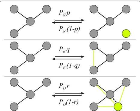
Our networks are usually generated from a single seed node, but can take any specified initial configuration of nodes and edges as starting condition. Subsequent events, determined by user-chosen probabilities, occur stochasti-cally and usually lead to network growth. For example, the node-event probability P_N determines that a node is either added (without edges) or deleted, depending on a second parameter, the node addition probability p. Thus, for a single node event, the probability that a node will be added is pP_N while the probability that a node will be deleted is P_N (1-p) (see Figure 1). A second type of event affects edges with probability P_E: the edge-event probabil-ity. Just as with nodes, edges will be added with an edge-addition probability q, so that a single edge event will add an edge with probability qPE while an edge is removed

with probability (1-q)P_E. Note that while node addition or removal happens unconditionally, edge addition or

removal is not guaranteed. The algorithm will only place an edge if the pair of nodes that is randomly selected is unconnected. Similarly, an edge removal instruction is only carried out if the pair of nodes that is randomly selected already has a connection, and otherwise fails. As a consequence, even edge addition probabilities q < 0.5 will lead to a steady-state distribution of edges to nodes. The main parameters of the growth model are summa-rized in Table 1. Note that because a rescaling of the probabilities pP_N, qP_E, and rP_D by a common factor only changes the time it takes to achieve a network of a partic-ular size, these probabilities are not independent (for example, pP_N can be used to rescale all parameters). How-ever, for many applications it is interesting to vary these probabilities independently.

We can calculate the steady-state distribution of edges per node (mean degree 冬k冭) by calculating the total num-ber of nodes n and edges m as a function of the number of events N and the parameters P_N, P_E, p, and q (we do not consider duplications in this calculation). The number of nodes added per event is pP_N and the number of nodes removed is (1- p)PN, so that the net number of nodes

added after N events

The net number of edges m added is more complicated, because edges are only added with probability q(1 - ξ), and removed with probability (1 - q)ξ per event, where ξ

is the graph sparseness , and represents the

probability that a random pair of nodes is connected by

n=NP_N(2p−1). (1)

x = _{n n(}2m₋₁₎

Table 1: Parameters of network growth model

Abbreviation probability

PN Node-event probability PE Edge-event probability PD Duplication-event probability

(duplication or fusion) p Conditional node-addition

probability (given a node event). Conditional probability of node removal is 1 - p

q Conditional edge-addition

probability (given an edge event). 1 - q is the conditional probability that an edge is removed

r Conditional node-duplication probability (given a duplication/ fusion event). Conditional node-merging probability is 1 - r

an edge. At the same time, every time a node is removed,

the algorithm removes the edges attached to it. On

aver-age then, a node removal event subtracts the averaver-age

degree of that node, which is iki/n = 2m/n = 冬k冭, so that

We can then write an equation for the asymptotic dependence of the mean degree

or

where η = PE/PN, and using ξ ≈ 冬k冭/n, which holds for

large n. Thus we see that in the limit of large n,

a behavior that is borne out in the simulations (data not shown).

A third type of event leads to node duplication or merger (fusion), controlled by the parameter P_D. Here, a node is duplicated with probability rP_D, while two nodes are fused with probability (1 - r)P_D (the parameters are summarized in Table 1). While edge and node events are straightforward, node duplication/fusion events need more explanation because there are several different ways in which nodes can be duplicated or fused. Here, we implement an algorithm in which node duplication is directly related to the concept of modules: When dupli-cating a node, the new node is by definition in the same module as its ancestor, and the new node is connected to all nodes the ancestor is connected to. In order to imple-ment this, nodes have to be assigned a tag that deter-mines the module they belong to, the moment the node is created. (It is convenient to represent different tags by different colors, so we often refer to nodes in different modules-that is, carrying different tags-as having differ-ent colors).

In order to assign a module to a duplicated node, the

number of modules has to be given at the outset, and the

probability for a node of color k to connect to a node of color ᐍ is obtained from the assortativity matrix e, which stores the fraction of edges between pairs of colors. For

N_c modules M₁,..., , this matrix can be written as

For the case of node merging, two nodes (A and B) are picked at random. Node A keeps its connections and in addition obtains all the connections that node B had, upon which node B is deleted. The selection of the nodes to be merged is module independent, and thus could either merge nodes within a module or across modules.

When growing modular networks, nodes are assigned a color based on a vector of probabilities that can be speci-fied beforehand (for all the results in this paper, nodes are assigned to a module randomly at the time they are cre-ated). If an edge event specifies the placement of an edge, a random pair of nodes is selected and the identity of the colors determined. At this time, a random uniform num-ber is drawn, and the edge is placed if this numnum-ber is smaller than the corresponding probability in the e -matrix (6). If no edge is set, the algorithm tries to set the edge for a different pair of nodes, and attempts this up to 1,000 times.

We determine a growth stop criterion either by specify-ing a maximum number of nodes, or by specifyspecify-ing a fixed number of iterations of the algorithm. In principle, the algorithm allows for the generation of both directed and undirected graphs. Here, we restrict ourselves to net-works with undirected edges, and furthermore prevent nodes from connecting to themselves. Finally, two differ-ent growth initial conditions are possible: one in which we start with a single node from the first module in the e -matrix, the other where we start with a single node from every module. The N_c(N_c - 1)/2 entries in the assortativity matrix, together with the number of colors and the six probabilities for stochastic network growth described above fully determine the structure of the network.

Software availability

The program to grow the networks described in this arti-cle will be made freely available.

Results and Discussion

Growing networks with complex degree distributions The standard model for growing graphs with exponential degree distribution is due to Callaway et al. [43], who introduced a model where a node is added at each event, and an edge is added with a given probability per event. While there are no duplications in this model and edges are not preferentially attached to high-degree nodes, there is still a form of preferential attachment because older nodes have had more opportunities of obtaining

m=NP q_E( −x)−NP_N〈 〉 −k(1 p). (2)

〈 〉 = = − − 〈 〉 −

−

k m

n

PE q PN k P

PN p

2 2 2 1

2 1

( ) ( )

( )

x

(3)

〈 〉 ≈ +

k q

n

2 1 2

h

h/ , (4)

〈 〉 →k 2hq, (5)

M_N

c

e

p M M p M M p M M

p M M p M M p M M

N

N

c

c

=

→ → →

→ → →

( ) ( ) ( )

( ) ( ) ( )

1 1 1 2 1 2 1 2 2 1

… …

pp M( Nc M) p M( Nc M ) p M( Nc MNc)

.

→ → →

⎛

⎝ ⎜ ⎜ ⎜ ⎜ ⎜

⎞

⎠ ⎟ ⎟ ⎟ ⎟ ⎟

1 2 …

edges, and also have a higher probability of connecting to nodes with more edges [43]. This model produces expo-nential degree distributions whose form can be predicted exactly, but scale-free distributions cannot be produced. With the present network growth model, it is easy to grow networks with more complex degree distribution, by changing just a few parameters.

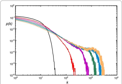
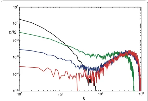
To begin with, we test whether the exponential distri-bution of the Callaway model morphs into a scale-free distribution as the duplication event probability is increased. In Fig. 2 we show the degree distribution with a fixed node and edge event probability, but changing the node duplication probability P_D, and confirm that if net-works grow with duplication, the scale-free edge distribu-tion is unavoidable [41]. Networks that are scale-free over more decades actually emerge if nodes are added more often than edges (see Fig. 3A). Choosing a low P_N, on the other hand, leads to the growth of networks with a Pois-son-like degree distribution (Fig. 3B). Note that the scale-free and the Erdös-Rényi-type distributions depicted in Fig. 3 were obtained using the same set of parameters except that the node addition probability was 100 times less for the graph that resulted in an Erdös-Rényi-like edge distribution. In principle, keeping the relative ratio of the three probabilities P_N, P_E, and P_D the same (when p

= q = r = 1) results in the same edge distribution (see

Models and Methods).

Choosing probabilities in between the parameter values described allows us to grow very different networks, with edge distributions in between exponential and Poisson. For example, there are interesting "transition stages" where parameter combinations lead to networks that are

neither scale-free nor Erdös-Rényi. We show in Fig. 4 extreme and intermediate edge distributions where we varied the node-event probability (P_N) from 0.001 to 1.0 while keeping all other probabilities constant. The distri-bution obtained for P_N = 0.001 has all the characteristics of an Erdös-Rényi-type edge distribution, such as the one depicted in Fig. 2B (note the difference in scales). We conclude that the edge distribution can be controlled entirely with the node addition probability and the edge duplication probability (as long as the edge addition probability is not too low): for low edge duplication, tun-ing P_N from 1 to small values morphs the degree distribu-tion from exponential to Erdös-Rényi. If the edge duplication probability is substantial, however, the same change in P_N moves the distribution from scale-free to Erdös-Rényi. As a corollary, moving PD from small values

to larger values for moderate to high P_N changes an expo-nential towards a scale-free distribution, as we saw in Fig. 2. While we have not conducted an exhaustive parameter exploration, we can summarize how the main parameters affect the degree distribution in a qualitative manner. In the absence of duplication, the degree distribution is exponential or approximately Poisson, depending on the size of the ratio of the edge- to node-event probability η =

P_E/P_N and the edge addition probability P_D. For q = 1, the Callaway model [43] predicts an exponential edge proba-bility distribution

with mean number of edges per node (degree) 冬k冭 = 2η

in agreement with Eq. (4) (see Fig. 5 center). If η becomes large, however, this distribution starts to resemble a Pois-son distribution, as indicated in Fig. 5. An Erdös-Rényi-type distribution can also be obtained without touching

η, by simply decreasing q (the probability that a node is added per edge event) because as long as edges are added slowly, a small enough q will lead to the random rewiring of a graph (see Fig. 5 lower left). In both cases (η Ŭ 1 or q

< 1 while η ≈ 1) the edge probability distribution quickly becomes independent of the network size. As we increase the node duplication probability, we move towards the distributions on the right hand size of Fig. 5. While the distribution starts to develop a form reminiscent of a power-law for low degrees when η < 1, the duplications lead to a hump at larger degrees. Whether or not this dis-tribution is independent of the size of the network is unclear: when duplications enter the generation process, may of the graph properties depend not only on the initial configuration used for the graph, but also the length of the process. Likewise, it is unclear whether the parame-ters that give rise to power law distributions for a finite

p k

k

k

( ) ( )

( )

=

+ +

2

1 2 1

h

h

(7)

Figure 2 Degree distribution as a function of duplications. The de-gree distribution of randomly grown networks with different node du-plication probabilities P_D (r = 1), at fixed P_N = 0.2, P_E = 0.75 (with p = 1, q = 1). PD = 0 (black), PD = 0.1 (red), PD = 0.2 (magenta), PD = 0.3 (green), PD

= 0.4 (blue), and PD = 0.5 (yellow). Average of 100 replicates of networks

process (as in the lower right graph in Fig. 5) are the same if the size of the network tends to infinity. Fortunately, real-world networks are not infinite, so the model is use-ful for the generation of surrogate networks even if the asymptotic distribution is not known.

The algorithm can be used to create lattices with an arbitrary degree or connectivity by making use of the assortativity matrix in an unconventional manner: Each node of the lattice is assigned a unique module, where the probability of having an edge between modules reflects the desired neighborhood relations in the lattice. Instead of seeding the growth process with a single node, the

algorithm is started with a fixed number of nodes and no edges, and P_N = 0. The growth process then enacts a per-colation problem with edge probability qPE, and a

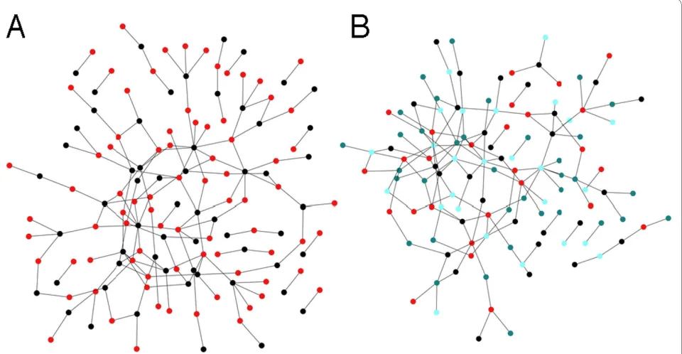
geome-try dictated by the assortativity matrix. To create bipartite graphs with edges only connecting nodes from different groups, we can grow networks from an assorta-tivity matrix with a vanishing diagonal [see Fig. 6A]. Nearly bipartite graphs are obtained by varying the entries in the matrix accordingly. Clearly, the algorithm can generate arbitrary k-partite graphs, by extending the dimension of the assortativity matrix. We show in Figure 6B a network iterated for 1,000 steps with the same parameters as Fig. 6A, but with k = 4 (nodes colored according to the group label).

Modularity

That biological, technological, and social networks are organized in a modular fashion is by now a commonplace observation. Yet, there is no standard measure of modu-larity, nor is there a standard algorithm that will partition networks into modules. There are several reasons for this apparent shortcoming. On the one hand, while the term "modular organization" is fairly intuitive, anyone who is familiar with the structure of real-world networks under-stands that this intuitive notion can only be applied approximately, and with a good amount of prudence. Modules are often identified using the topological struc-ture of the network, for example by counting the number of shortest paths between nodes, or by identifying an excess number of edges between nodes as compared to a random (Erdös-Rényi-type) network. However, it is also possible that groups of nodes function together as a mod-Figure 3 Edge distribution of networks grown with different parameters. (A) Scale-free edge distribution p(k) of networks obtained with a growth algorithm using PN = 0.2625, p = 1.0, PE = 0.15, q = 1.0, PD = 0.225, and r = 1.0, undirected edges, no modules, average over 1,000 networks grown

to 10, 000 nodes. (B) Edge distribution of networks grown with PN = 0.002625, all other parameters as in (A), averaged over 10,000 networks grown to

1,000 nodes.

Figure 4 Edge distributions for networks grown under different regimes. P_N = 1.0 (black line, exponential distribution) P_N = 0.1 (green), PN = 0.01 (blue), and PN = 0.001 (red). All other parameters are set to PE

= p = q = 0.75, PD = 0.5, r = 1.0. Networks are unmodular and undirected,

ule without any obvious topological signature. Further-more, functional modules often overlap, while topological modules are usually defined in such a way that they are mutually exclusive. Therefore, we expect that topological and functional measures of network

modularity can disagree, and that this disagreement can be more or less severe depending on the type of network under consideration.

We would also like to highlight the difference between modularity measures, which quantify the modularity in a Figure 5 Changing a network's degree distribution. This sketch indicates how different degree distributions morph into one another as several different parameters of the growth model are changed. From the "default" exponential degree distribution of the Callaway model (center of diagram) Erdös-Rényi-like distributions can be obtained in two different ways: either by increasing the probability to add edges while keeping the node addition probability constant, or by randomizing edges using a small q (distributions on the left, note the non-logarithmic axes). Approximately scale-free dis-tributions can be obtained from the exponential one by increasing the node duplication probability, but doing so while decreasing the number of edges per node creates a hybrid between scale-free and Erdös-Rényi-type distributions (distributions on the right).

η >> 1.0

q < 1.0

η ~ 1.0

P ~ 0.3

η < 1.0

P > 0.0

η = 1.0

q = p = 1.0

P

= 0

D D

Figure 6 Bipartite and k-partite graphs. (A) Bipartite graph, nodes from one group colored in red, nodes from the other group colored in black, PN/

PE = 0.3, p = 0.85, q = 0.75, PD = 0.0. The graph was grown for 1,000 iterations of the algorithm, with undirected edges. (B) Graph grown with the same

network whose modules have already been determined, and module-discovery algorithms, which partition a net-work into groups of nodes. Often, module-discovery is performed by attempting to maximize a modularity mea-sure, but in principle neither does a modularity measure imply an algorithm for module discovery, nor does a module-discovery algorithm necessitate a measure of modularity.

A commonly used measure of modularity is due to Newman [17], who assumes that modularity implies that nodes in the same module have more connections between them than would be expected for a random con-trol, that is, a network where all the module assignments have been randomized. If k_i is the number of edges of node i, and m = 1/2 _i k_i is the total number of edges in the network, then the probability that two nodes i and j are connected by chance is k_ik_j/2m (as long as the degrees for node i and j are independent). Now, define the network adjacency matrix A, in such a way that A_ij = 1 if node i

connects to node j and Aij = 0 otherwise. This matrix is

symmetric for undirected networks, and can have non-integer entries if the strength of a connection is taken into account. Here, we limit ourselves to undirected networks that have "binary" edges, but the extension is obvious. We furthermore limit ourselves to networks without node self-connections, which implies that the diagonal of A

vanishes. If furthermore the module assignment for each node is known, we can define a modularity matrix S in such a way that S_ij = 1 if nodes i and j belong to the same module, and zero otherwise. Newman's modularity Q_N is then defined as [17]

There is clearly a certain amount of arbitrariness in modularity measures of this kind. For example, a different measure using similar ideas is often called the "assortativ-ity" of a network. This measure is also due to Newman [25], and quantifies how likely it is that nodes of the same "kind" attach to each other, where "kind" can be any tag that is attached to a node to distinguish it from another class of nodes. As before, we refer to this tag as the node's color, so that assortativity measures how often nodes of the same color connect to each other rather than to nodes of a different color. Let us define the assortativity matrix e

(sometimes called the "mixing matrix") such that e_kᐍgives the fraction of edges that attach a node of color k to a node of color ᐍ, and ak = ᐍekl is the fraction of edges that

either begin or end at a node of color k (we again restrict ourselves to undirected networks here, so that e is sym-metric). Newman's assortativity is then given by [25]

Both measures (8) and (9) are bounded from above by 1, and they can both become negative (indeed, Newman's modularity and assortativity measures are closely related, see Appendix). While the assortativity is constructed in such a way that networks with random assignment of col-ors (modules) to nodes gives rise to a vanishing measure, this is not generally true for Q_N. Furthermore, both mea-sures can in principle detect in networks a tendency of nodes of the same module or color not to connect to each other (a phenomenon we call anti-modularity or anti-assortativity). However, the measures do not treat anti-modularity (or anti-assortativity) on the same footing as modularity or assortativity.

It is possible to introduce a measure of modularity that is closely related to both of Newman's measures, but gives more weight to "like"-edges if the number of colors is large. This is obtained by modifying the modularity matrix that enters Eq. (8) so that

where N_c is the number of modules or colors. (As in the following we will tag nodes that belong to the same func-tional module with the same color, we often refer to col-ors or modules interchangeably.) With such a modularity matrix, connections between nodes of unlike color are penalized, most heavily so if there are only a few colors. We define our functional modularity measure in terms of this generalized modularity matrix

but note that we omitted the term -kikj/2m in

New-man's measure that subtracts the probability that two nodes connect at random. Indeed, the latter bias is typical for modularity measures that attempt to capture the way modules are reflected in network topology, while our measure Q_H focuses on function only. Because Q_H can also be written as (see Appendix)

Q

m A

kik j

m S

N ij

i j

ij

= ⎛ −

⎝

⎜⎜ ⎞_⎠⎟⎟

∑

1

2 2

,

. (8)

r e k ak

k ak

= −∑

−∑

Tr 2

1 2

. (9)

S

i j

N c

ij = ₋

− ⎧ ⎨ ⎪

⎩⎪

1 1

1

if in same module as

otherwise,

(10)

Q

m_{i j}AijSij

H = ∑

1

2 _, , (11)

Q N c

N c e N c

H = ₋ −

⎛ ⎝

⎜ ⎞

⎠ ⎟

1

1

we see that Q_H vanishes for non-associative (non-mod-ular) networks, because when color is assigned randomly

to nodes we have so that Tr e = 1/N_c. At the

same time, Q_H is maximal for graphs if colors only con-nect to like colors (Tr e = 1). But in contrast to Newman's measures, Q_H can become significantly negative, more so if the number of modules is small. For bipartite graphs,

for example (graphs with nodes of two colors where only

unlike colors connect) we find Tr e = 0, so that Q_H = -1. To study how the different modularity measures depend on the number of modules in the network as well as the strength of the module's interconnectivity, we gen-erate networks with a tunable amount of modularity. A simple model for generating modular networks is an assortativity matrix for Nc colors where like-colors

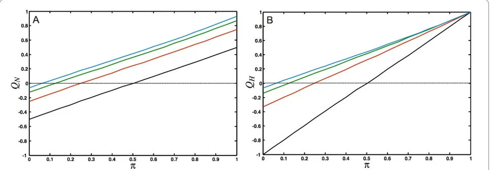
con-nect to each other with probability π (the intra-module edge probability), and connect to nodes of a different color with probability (1 - π)/(N_c - 1), irrespective of color (the "equal opportunity" model, see Appendix). The prob-ability 1 - π can then be viewed as an inter-module edge probability and can be used to dial between perfectly modular (π = 1) and perfectly anti-modular (π = 0) net-works. The functional modularity Q_H seen in Fig. 7B depends strongly on the number of modules, and is larger than Q_N (depicted in Fig. 7A) for modular networks, and smaller than Q_N for the anti-modular ones. Indeed, the inherent bias in Newman's measure for modules whose member nodes are strongly connected to each other leads

to an underestimate of the modularity for strongly con-nected modular graphs, and an equally underestimated antimodularity for multipartite graphs, as compared to the measure Q_H, when the number of modules is small. The functional measure Q_H, in turn, cannot be used to

detect the number of modules or communities, for pre-cisely this reason: because no connection bias is assumed, there are no topological means to identify clusters. If the number of modules is given, on the other hand, Q_H can be used to guide a graph partitioning algorithm. Note that the measures become indistinguishable in the limit of an infinite number of modules.

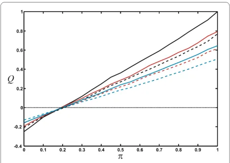
We can also investigate the impact node fusion has on modularity (Figure 8), for the modularity measures Q_N

and QH, by studying how modularity depends on module

strength in networks grown with different node fusion probabilities. Irrespective of the measure, modularity is highest if nodes are not fused (r = 1) and decreases as the node fusion probability increases (r < 1) because node fusion is blind to the module assignment, while node duplication creates another node with the same color and the same edges as the original node. The larger the proba-bility for adding an edge within modules is (larger π), the more modular the networks are, as expected. Because Q_H

does not penalize modules if they do not have an excess of edges between them, Q_H is mostly larger than Q_N. For small π, more connections exist between nodes of differ-ent modules than within them, so that both modularity measures become negative.

The impact of node duplication on modularity is more complicated. On the one hand, because node duplication brings with it the duplication of the edges that the

dupli-e_ij=1/N_c2

Figure 7 Comparison of modularity metrics. Comparison of the modularity measures defined in Eqs. (8) and (11). Networks with between 2 and 16 modules were grown depending on the intra-module edge probability π. (For π = 0 the networks are as anti-modular as possible and become k-partite (where k is the number of modules), while for π = 1 they are as modular as possible). (A): Q_N [defined in Eq. (8)] for N_c = 2 (2 modules, black line), N_c = 4 (red), Nc = 8 (green), Nc = 16 (blue). (B) QH [defined in Eq. (11)]. Colors as in (A). Each point was averaged over 50 networks with 1,000 nodes. The

cated node is attached to, whether or not node duplica-tion leads to an increase in modularity depends on whether the network sports more inter-module or more intra-module edges. On the other hand, node duplication can skew the fraction of nodes that belong to any particu-lar module by amplifying stochastic events that occur early-on in network growth. While node colors are cho-sen either randomly or according to a node probability vector when a node is created (see Model), the color of a node (that is, its module membership) is inherited under duplication. As a consequence, module sizes fluctuate considerably across different realizations of the network, and the modularity can become significantly different from that predicted by the e-matrix generating the net-work. A detailed analysis of duplication on modularity is beyond the scope of this manuscript, and will be pre-sented elsewhere.

Global properties

A number of interesting global topological properties have been observed in networks, both in the case of bio-logical or engineering networks that are built via growth processes, and in Erdös-Rényi-type networks that form via random edge addition. Foremost in the first category is the "small-world" effect: the observation that many bio-logical and technobio-logical networks have a short mean path between nodes (as compared to an equivalent ran-domized network), while being highly clustered (again with respect to a randomized equivalent network [52], see also the review [53]). Humphries and Gurney [53] introduced a quantitative measure to study the "small-world-ness" of a network, which is particularly useful

because networks that have a high edge-density can auto-matically appear to be in the small-world class, but trivi-ally so. Following Humphries and Gurney, we define the ratio of the "mean shortest path between nodes" in a net-work to the mean shortest path in the randomized ver-sion of the network (an Erdös-Rényi network with the same number of nodes and edges):

and the ratio of the graph clustering coefficient

with respect to that of the randomized version

The symbol Δ in the superscript of the clustering coef-ficients serves to remind us that this coefficient is obtained by counting the number of "triangles" of nodes normalized to the number of pairs [54], which can be dif-ferent from the clustering coefficient obtained by averag-ing the number of edges of the adjacent nodes [52].

As small-world networks are identified by having a large γ_g and a small λ_g, the ratio of these quantities can be used to measure small-world-ness:

We show the behavior of λg and in Fig. 9 as a

func-tion of the ratio of node- to edge-event probability P_N/P_E

for networks grown to a size of 200 nodes. As more and

more nodes are added per edge-addition event

(increas-ing ratio P_N/P_E towards 1), the normalized mean shortest path first drops, and indeed, as long as P_N/P_E < 1.5 (for q = 1), the shortest paths in these networks are shorter than those in randomized networks. But once passed this

threshold, the addition of more nodes without a

com-mensurate increase in edges leads to longer and longer

shortest paths (see Fig. 9, solid red line). The normalized

correlation coefficient increases rapidly with an

increas-ing ratio P_N/P_E up until P_N ≈ 0.65P_E, after which the ratio drops very fast.

lg L g

L =

random

, (13)

C_gΔ C_randomΔ

gg

C g C

Δ Δ

Δ =

random

. (14)

S g

g Δ ₌gΔ

l . (15)

ggΔ

Figure 8 Modularity depends on node-fusion probability. Aver-age modularity (from 50 independent networks with five modules, grown to 1000 nodes) for different node duplication probabilities r = 0.5 (blue), r = 0.75 (red), and r = 1.0 (black), for the modularity measures QN (solid lines) and QH (dashed lines). The networks were grown with

We also tested how decreasing the conditional

edge-addition probability q affects λ_g and . We expect that a decrease in q will move the mean shortest path and the correlation coefficient towards their randomized graph

equivalents, because a q < 1 implies that sometimes edges are removed (for q = 1/2 edges are added as often as they are removed during an edge event), and the edge

removal/edge addition process is tantamount to a

ran-domization of the graph. We do indeed observe that

TC_random as q decreases (we show the case of q = 0.75 in

Fig. 9), but L_g/L_random actually increases for decreasing q as long as PN/PE d 2.

In order to determine what graph-growth parameters give rise to small-world networks, we plot the ratio SΔ

defined in Eq. (15) (which is just the ratio of the two curves depicted in Fig. 9) as a function of the ratio P_N/P_E

(Fig. 10). In this figure, we also plot the edge density (or "sparseness") of the network (here m is again the number of edges, and n the number of nodes in the network)

because it is known that networks with a high density of edges can be trivially of the small-world kind [53]. We see from Figs. 9 and 10 that networks grown with a ratio

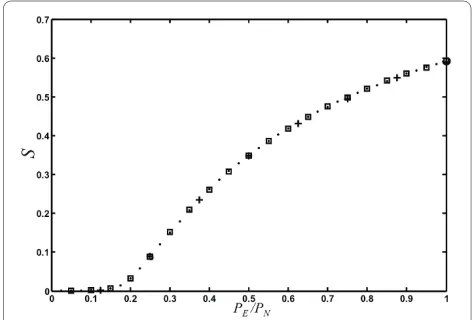
P_N/P_E < 1.3 have a small-world character, and further-more that this character is maintained even for small ratios P_N/P_E down to about P_N/P_E ≈ 0.2, where the edge density is ξ ~ 0.1. This behavior is similar to that observed in the Watts-Strogatz model [52], which becomes "trivi-ally small-world" in the limit of increasing randomness [53].

Figure 10 suggests that networks with small-world character are an automatic by-product of a stochastic growth process where the edge-event probability is of the order of the node-event probability or larger (here, P_E/P_N

t 0.75), while the small-world character becomes trivial if

PE is many times PN. This is a plausible scenario for a

number of biological networks, where it is much more likely to create a new edge (for example, an interaction between two proteins via a gain-of-function mutation, or a regulatory interaction) than it is to create a new node (the evolution of a new protein de novo or via lateral gene transfer). We can also see that this regime is easily achieved in social networks, as long as the creation of an interaction between nodes is more common than the addition of a new member to the social network.

Critical behavior

Besides degree distribution, modularity, and small-world-ness, a number of other global properties of networks have been studied in the literature that we can study with ease using our network growth model. It is known since the pioneering work of Erdös, Renyi, and Bollobas that static random graphs undergo a phase transition where a "giant component" (a large connected component that scales with the size of the system) emerges at a critical probability of connecting edges (see, e.g., [55]). This

g_gΔ

C_gΔ

x = −

2 1

m

n n( ), (16)

Figure 10 Small-world-ness SΔ as a function of PN/PE. The quanti-tative measure of small-worldness SΔ _{(solid line) and the edge density}

ξ [Eq. 16] (dashed line) as a function of the node to edge addition prob-ability ratio. Networks are non-trivally "small-world" if SΔ _{> 1 while the}

edge density is low (e.g., ξ < 0.1).

Figure 9 Normalized mean shortest path and correlation coeffi-cient. The normalized mean shortest path between nodes, Lg/Lrandom

(red lines) and the normalized correlation coefficient

(blue lines) as a function of the ratio P_N/P_E, for a node

duplication probability p = 1 and two different edge addition probabil-ities q = 0.75 (dashed) and q = 1 (solid). Average over 1,000 networks grown to 200 nodes, with P_D = 0.

phase transition is of the same kind as in percolation models, and is often referred to as the percolation transi-tion in random graphs. Callaway et al. [43], Dorogovtsev et al. [56], as well as Bollobas et al. [57] have pointed out that random networks that are grown also undergo a per-colation transition, but that this transition has a very dif-ferent character: the critical point is infinitely differentiable (in fact, all the derivatives vanish at the crit-ical point [43,56,57]). We can study this transition in our model as a function of parameters not previously investi-gated, namely P_N, p, q, as well P_D and r. We observe that the percolation phase transition only depends on the ratio P_E/P_N (see Fig. 11), that is, the size of the giant com-ponent S only depends on the relative rate at which nodes and edges are added. Even varying q (allowing for edge removals) does not change this transition, as long as we plot the giant components versus qP_E/P_N instead (results not shown). Note that this combination of parameters is related to the asymptotic mean degree 冬k冭 (see Eq. (5) in

Models and Methods).

Similarly, allowing for node duplication does not change the transition, as duplications may change the absolute size of the giant component, but do not affect its emergence. Node fusion, on the other hand, does affect the emergence of the giant component because fusions can lead to the merger of two separate clusters. We show in Fig. 12 the relative size of the largest connected com-ponent of networks grown with different node fusion probabilities (P_D = 0.0, 0.1, 0.25, 0.5, r = 0), where the value PD = 0 serves as the control (no node fusion). As

expected, the onset of the transition is earlier when nodes can fuse, because node fusion does not change the giant component if the nodes are in the same cluster (except for

diminishing its size by one), whereas whole clusters are fused if the nodes that are fused belong to different clus-ters. The nature of the phase transition (infinitely differ-entiable critical point) is unchanged. Of course, as nodes are fused, the network grows more slowly, but the shape of the curve in Fig. 12 cannot be recovered simply by scal-ing P_N and P_E taking into account the modified number of nodes and edges for each fusion event (data not shown).

Biological relevance

Given the variability of the networks that can be gener-ated with this model, we may ask whether it is universal in the sense that the edge distribution of any biological network can be characterized by the set of parameters (five independent constants plus the e-matrix). We tested whether networks can be grown to have an edge distribu-tion that is similar to well-known biological reference examples, and whether the set of parameters giving rise to these networks allows us, by analogy, to generate hypotheses about the process that generates them. Spe-cifically, we grew networks to resemble the edge distribu-tion of the neuronal network of the nematode C. elegans

[58], as well as a network similar to the protein-protein interaction network of yeast [59]. The best current data set for the C. elegans "brain" includes 280 of the 302 neu-rons and their connections [58]. We binned the edge dis-tribution from this data set and searched the parameter space of the model (five parameters, no modules, undi-rected edges) for sets that grow networks of 280 nodes with an edge distribution that minimizes the root mean square difference of the corresponding binned edge dis-tribution. Note that because a graph's properties are Figure 12 Percolation phase transition with node fusion. The rela-tive size of the largest connected component S as a function of the rel-ative edge to node event probability (with p = 1, q = 1, and r = 0), for different node fusion probabilities (as r sets the node duplication prob-ability, the fusion probability (1-r)P_D is simply given by P_D). Solid line: P_D = 0, dash-dotted: P_D = 0.1, dashed: P_D = 0.25, and dotted: P_D = 0.5. Aver-age of 100 replicates of networks grown to size n = 100.

Figure 11 Percolation phase transition in randomly grown net-works. Relative size of the giant component S as a function of P_E/P_N, for networks grown with various combinations of PN and PE: Crosses: PN =

0.1, circles: PN = 0.2, squares: PN = 0.5, dots: PN = 1.0 (with PD = 0 and p =

unchanged if the relative ratio of the three event probabil-ities is maintained (as long as neither of them becomes too small), we kept the largest of the parameters (here P_E) fixed. We verified that a search with six independent parameters gives rise to the same set if rescaled to P_E = 1.

Within the space of network parameters, the C. elegans

network appears to be fairly rare, so that a straightfor-ward Monte Carlo search often arrives at inferior fits. Our best solution is a network with P_N = 0.008, p = 0.71,

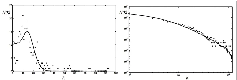
P_E = 1.0, q = 0.06, P_D = 0.028, r = 1.0 (P_E was fixed at 1.0 in this search). We show the degree distribution generated with this set of parameters (averaged over 1,000 realiza-tions of the network) in Fig. 13A (solid line). A statistical test comparing these distributions cannot reject the hypothesis that they were generated from the same underlying probability distribution (Wilxocon rank sum test, P = 0.744). This set of probabilities suggests that the

C. elegans network reflects a growth process with a very small node addition probability, commensurate with our earlier observation that networks with an Erdös-Rényi-like degree distributions are obtained using a small PN.

Such a small node addition probability is also consistent with the constraints imposed on C. elegans evolution by its invariant cell-lineage. The worm develops via stereo-typed cleavages so that the patterns of cell division, differ-entiation, and death are the same from one individual to another: in the developing worm each cell has a predict-able future, and each cell a well-defined set of neighbours [60]. As a consequence, developmental changes giving rise to new nodes must be heavily constrained, as they would upset the delicate balance. For the same reason, node duplications are also virtually absent in the simu-lated network. The small edge addition probability q =

0.06 implies that edges are only added in 6% of the edge events, and the network is consequently quite sparse. As the algorithm does not remove an edge if there is none between the randomly selected nodes, even such a small edge addition probability (in fact, it corresponds to a 0.94 edge removal probability) always gives rise to an equilib-rium edge count (calculated in Models and Methods in the absence of duplication).

The simulation of the yeast protein-protein interaction network (interaction data from the highly curated set of Ref. [59]) leads us to vastly different conclusions concern-ing the nature of the growth process. Because this net-work is much less rare, a Monte Carlo search converges fairly rapidly, and yields a similar set of parameters in all trials. For yeast, we started with 4 different initial condi-tions, conducted 5 trials each, and grew 20 replicas for each parameter set to obtain an average distribution, which we score by comparing the root mean square dif-ference of the binned distribution to the binned yeast dis-tribution. Because of the sparseness of the data at high degrees, we performed a "threshold-binning" with vari-able bin size, as described in [61]. We stop growth at 3,306 nodes (the size of the Reguly et al. network) and obtain a network that is remarkably similar to the yeast protein-protein interaction network, with P_N = 0.7 ± 0.04,

p = 1.0 ± 0.05, P_E = 1.0 ± 0, q = 0.91 ± 0.035, P_D = 0.75 ± 0.035, r = 1.0 ± 0.03. A statistical test comparing the yeast degree distribution and that of our simulation for nodes with less than 120 edges (see Figure 13B) cannot reject the hypothesis that both distributions were obtained from the same underlying process (Wilcoxon rank sum test, P = 0.0837). The eight proteins in the yeast network with more than 120 nodes appear to be outliers that do

not follow the same law as the remaining 3,298 proteins in the network.

Both the node addition probability P_N and the node duplication probability P_D creating our surrogate yeast network are remarkably high. That the node duplication probability is this high for the generation of a protein-protein interaction data set is not surprising in the light of evidence that much of genomic evolution proceeds via gene duplication and subsequent diversification [62,63]. However, the analysis also suggests that the yeast network edge distribution is only very approximately scale-free.

We conclude that particular degree distributions are (at least for the cases we examined) obtained with unique parameters sets, thus allowing us to entertain hypotheses about the processes that generated the networks we are simulating. Of course, such speculations rest on the assumption that other processes (such as for example, whole genome duplication, or horizontal transfer of sets of genes) do not play a role in shaping the network's edge distribution. Because we cannot rule out such processes in many of the standard networks, such a caveat always has to be issued.

Conclusion

We have presented an algorithm that, using only a few parameters, can generate networks of seemingly arbitrary degree distribution, modularity, and structure. Using this model, we were able to study how fundamental proper-ties such as edge addition or removal, as well as node addition, removal, duplication, or fusion, affect a net-work's degree distribution, modularity, and structure. We found that we could grow networks with degree distribu-tions anywhere between binomial, exponential, and scale-free, within a single framework or process. By introduc-ing an assortativity matrix for the generation of nodes with different functional tags, we could furthermore grow networks with different degrees of modularity, by speci-fying the probability that a node of one "color" will attach to a node with a different color. Once modules or func-tional groups have been identified in any real network, control networks can be grown that mimic the connec-tion pattern or modularity of that network. One obvious example is again the C. elegans neuronal network. Its nodes can be divided into three classes: sensor neurons, motor neurons, and interneurons [58]. The e-matrix for this network can be reconstructed from the frequencies of inter-color edges, and be used to grow networks that not only have the same degree distribution as the original network, but mimic the connection pattern between functional types as well.

We also introduced a modified modularity measure Q_H

for networks that is based entirely on the functional char-acterization of a network's nodes, rather than the

connec-tion pattern. This measure is neither better or worse than any of the existing modularity measures (such as New-man's Q_N or the assortativity r), but rather highlights a different aspect of modularity. For example, while New-man's modularity Q_N defines modules as those groups of nodes that are connected to each other more often than would be expected from the connection probability in a random graph of the Erdös-Rényi-type, the measure Q_H

does not assume such a bias. In fact, because most bio-logical, social, and technological networks are not of the Erdös-Rényi-type, it is often erroneous to compare the connection probability of modules to what would be expected in a random graph. This is particularly true for networks with scale-free edge distribution, which sport a number of hubs with many edges that do not necessarily connect to other nodes within the same module. The measure Q_N will attempt to join such hubs in one and the same module, even if a measure based on betweenness centrality will separate them (see Appendix). QH, in

con-trast, does not allow you to detect modules, but rather quantifies the modularity of a graph based entirely on a previous group identification. Using such a measure, we can show that graphs are often less than modular, and can even become modular. An extreme case of anti-modularity is given by bi-partite, and by extension, k -par-tite graphs. In fact, precisely modular and k-partite graphs appear as "dual opposites" in this framework, obtained with an e-matrix with only ones on the diagonal and zeros elsewhere (divided by the number of modules), or else zeros on the diagonal for the k-partite graphs.

converged to suggest a unique set of parameters for each of those networks that led to biological conclusions com-patible with our current knowledge about the forces that shaped these networks. We expect this model to be most useful in the generation of null models in the analysis of biological, technological, and social networks. The pro-cess easily generates networks with the same size and degree distribution as any study network, but unlike the method presented in Ref. [64], the present process relies explicitly on network growth and can accommodate arbi-trary node "colorizations" (functional categories). Another standard control, the edge randomization of any network, is easily implemented by setting P_N = 0, P_E = 1, q

= 0.5 (with P_D = 0). This setting will remove and place edges randomly while keeping the total number of edges and nodes the same, resulting in a randomized graph after a sufficient number of updates.

We have shown that a broad set of standard results in network analysis, concerning the edge distribution, mod-ularity, global network structure, and critical behavior, can be reproduced in networks grown via a random pro-cess, with only a few tunable parameters. These net-works, however, were grown in the absence of any functional constraint, and their properties are therefore a consequence of the stochastic nature of the growth pro-cess only. We can conclude that while such properties may be useful for real-world networks, they are not nec-essary consequences of the network's functionality, but could simply be a consequence of how they emerged.

Appendix

Structural and functional modularity

Newman's modularity measure Eq. (8) can be shown to be related to his assortativity measure (9) by noting that the mixing matrix e is related to the adjacency matrix A

via a transform involving a matrix F that relates nodes to modules:

Introduce

Because , we find that

where the notation ||...|| indicates taking the sum of all the matrix elements. The mixing matrix e is then just

Noting that TrFFT _{= S, the modularity matrix defined}

above (8), we find that

The same construction also allows us to write Q_H

[defined in Eq. (11)] in terms of Tr e [Eq. (12)] by noting that

where 1 is a matrix where each entry is 1.

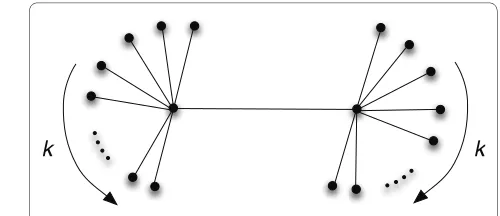
We can test the limits of the modularity measures (8) and (11) by calculating the modularity of an extreme graph as depicted in Fig. 14, which is a graph of two hubs of degree k connected by a single edge, and assuming that all of the nodes of one hub belong to the same module. In the limit of large k, such a graph should be classified as highly modular. However, Newman's measure applied to this graph gives

In comparison, the functional modularity measure Q_H, making the same assumptions about the modules, tends to 1 in the limit of high-degree hubs:

Functional modularity and assortativity

Newman's assortativity r [Eq. (9)] and the functional modularity measure Q_H [Eq. (11)] are identical for a par-ticular assortativity model, which we call the "equal opportunity" model. It is defined by the probability π for a

F_ki =⎧_⎨ i k

⎩

1 0

if node in module

otherwise . (17)

Ekl F A Fki ij jlT ij

=

∑

∑kFki= ∑lFjlT =1

E Ekl A m

kl

ij ij

=

∑ ∑

e Ekl

E m F A F

kl ki

ij

ij jl T

= = 1

∑

2 . (20)

Tr e

m A Sij

ij ij

= 1

∑

2 . (21)

S

N c S N

ij ij c

ij

= +

− − −

(1 1 ) ,

1

1

11 (22)

Q

k

N = − ₊ ⎯⎯⎯⎯_k→∞→

1 2

1

2 1

1

2. (23)

Q

k

H = −1 ₊ ⎯⎯⎯⎯_k→∞→

3 2

1

2 2 1. (24)

Figure 14 A graph with two hubs and k edges per hub.

color to connect to a node of the same color, but to con-nect to any other color with equal probability:

The factor 1/N_c, where N_c is the number of colors, serves to normalize e such that ||e|| = 1. It is easy to see that the fraction of nodes connected to type-k nodes: ak =

ᐍe_kᐍ= 1/N_c, so that (with Tr e = π)

which agrees with Q_H defined in Eq. (12).

Reviewers' Comments

Reviewer 1: Erik van Nimwegen, University of Basel This paper introduces an interesting parameterized class of stochastic network growth models that clearly can pro-duce networks with a range of different topological prop-erties, i.e., degree distributions, modularity, mean path lengths, clustering coefficients, as the parameters of the stochastic growth process are varied. It is quite conceiv-able that this parameterized family of growth models might actually be used to capture the broad topological properties observed in many 'real world' networks. This is very nice. However, what is a bit disappointing is that there are almost no analytical results on precisely what kind of properties the networks will have as one varies the parameters. All that is presented is a number of 'anec-dotal' examples of what one obtains with particular parameter settings. Moreover, the results are complex enough that one cannot easily generalize from the exam-ples presented. That leaves us in the end in a state where we have a family of growth models that MIGHT produce networks with desired properties, but it is unclear which kind of properties can be produced and precisely how to set the parameters to get them. That is, if I were to say: I have this real world network and it has this degree distri-bution, this distribution of distances between nodes, this distribution of clustering coefficients, and this modular-ity (according to whatever measure), then I don't think the authors could tell me whether there model could

pro-duce graphs with the same properties, and how to set parameters to get such graphs. In fact, the last section of the manuscript shows that, even to reproduce only the degree distributions of two biological networks, an expensive Monte-Carlo search is needed, and in the end the results clearly suggest that the growth model in fact cannot reproduce the observed degree distribution within statistical noise. This to me suggests that the prac-tical use of this family of growth models is extremely lim-ited until more general theoretical results about their behavior can be obtained.

Authors' response: First, we would like to thank you for the time you have spent reading our article, and assem-bling a long and detailed set of comments and questions. Many of your comments have led to important improve-ments in the presentation of the material. One of your main criticisms in the passage above, and repeated else-where in your comments, is a disappointment over the lack of a mathematical analysis of the graph growth model that we studied computationally. We have a good amount of sympathy for this position: it would be great to have a mathematical model that does all the things that you mention, and more. The problem with this is, also pointed out by you, that there are an infinite number of possible graphs, and there is simply no generative theory that could account for them all. Now, your suggestions for a mathe-matical theory sound less ambitious than that: you ask whether it would be possible to produce analytical results that will predict the form of the edge distribution, for example, given the input parameters, in the limit of infi-nite network size. This is at face value a reasonable propo-sition: after all, there is literature that predicts just that for a class of models that is a subset of the model described here. For example, it is possible to calculate the asymp-totic properties of graphs produced by a duplication model

[41]. But we wonder whether you are fully aware of how ambitious this proposition is. After all, deriving just the asymptotic degree distribution for a pure duplication model as in [41](which has a single parameter) is a ten-page publication. We have six main parameters (five of them independent, we will come to that), and possibly an infinite number of other parameters that allow us to spec-ify certain other aspects of the graph (such as the modular-ity) and even the adjacency matrix if we so desired. It is not that having a mathematical analysis of the sort that you wish you had seen would not be worthwhile having, it is just not the direction we chose to go because this is a tre-mendous undertaking that would take years of additional work. We have instead taken a much more practical approach. We understand that, for real systems, we will never know for sure what growth parameters have given rise to that network: even if we reproduced a particular biological network perfectly in all those properties that we can measure, we still could not state with certainty that e

N c

N c N c

N c N c

N c N c

= − − − − − − − − − − − − ⎛ 1 1 1 1 1 1 1 1 1 1 1 1 1

p p p

p p p p p p ⎝⎝ ⎜ ⎜ ⎜ ⎜ ⎜ ⎜ ⎜ ⎜ ⎜ ⎞ ⎠ ⎟ ⎟ ⎟ ⎟ ⎟ ⎟ ⎟ ⎟ ⎟ . (25)

r e k ak

k ak

N c N c

N c

N c N c

= −∑ −∑ = −− = − − ⎛ ⎝ ⎜ ⎞ ⎠ ⎟

Tr 2