Improvement Of Classification Accuracy For
Streaming Data Using Mtse Algorithm
Dr.Antony Selvadoss Thanamani, Padmapriya P, Malathi M, Sharmila S, Dr. A. Kanagaraj
Abstract: Ensemble based strategies are most generally utilized methods for classifying data streams. Their prominence is owing to their great execution when contrasted with solid single learners while being generally simple to convey in real time applications. For true issues, ensemble learning functions superior to traditional classifiers. This is valid for datasets with numerous examples closer to boundary of decision. Ensemble algorithms are particularly helpful for learning data streams as it can be coordinated with drift recognition calculations and consolidate dynamic updates, for example, specific evacuation or addition of classifiers. Utilizing meta-learner to learns from the expectations of base classifiers sums up better. Thus, Stacked Ensemble (SE) is favored over other troupe techniques. We broaden SE and introduce Multi-Tier Stacked Ensemble (MTSE) calculation with three tiers specifically a base tier, an ensemble tier and a generalization tier. Base tier utilizes the conventional classifiers for label prediction. 10-fold cross validation is utilized to approve the models in base tiers. The predictions cross validation are combined in next tier utilizing combination schemes. Ensemble tier predictions are generalized utilizing meta-learning to provide final prediction. At the point when examined with datasets, MTSE gives better execution over the stacked ensemble. It accomplishes maximum accuracy and isn't experiencing over-fitting/under-fitting.
Keywords: Stacked Ensemble, Incremental learning, MTSE, prediction, generalization, accuracy.
————————————————————
1 INTRODUCTION
The quantities of data produced by social networks, cellular phones and broad range of sensors have developed colossally. These data are just valuable if proficiently handled with the goal that people can settle on convenient choices dependent on them. A great progress is done in recent times, towards acquiring valuable models out of gigantic measures of quickly produced data in data stream mining. Data streams represent a few difficulties for learning calculations, including, yet not constrained to: fleeting conditions, concept drifts, enormous measure of occurrences, constrained labeled cases, feature drifts, novel classes, and confined resources (memory and time) necessities. Above all, issues found in batch learning setting are likewise present in context of data stream, e.g., missing values, noise, over-fitting, class unevenness, unessential features, and others. Ensemble learning consolidates the multiple weak classifiers predictions to give the final predictions [1, 2]. It enhances classification accuracy, stability and clout of the models. The ensemble performs better when base models accomplish over half of accuracy and are varied. Consequently the accuracy and variety of classifiers direct the viability of ensemble learning. All the precise models don't differ with various parts of information, and subsequently there is need to strike an ideal balance. There are 3 remarkable reasons for ensemble learning to be exceptional to conventional classifiers. They are (i) computational reasons (ii) statistical reasons & (iii) representational reasons. Instead of combining the outcomes from the powerless classifiers utilizing a static function like weighted or average sum, trainable combiners sum up well. These ensemble
frameworks are known as Stacked Generalization (SG) or Stacked Ensemble (SE). Here, combiner is additionally a classifier that is trained utilizing the labels anticipated by weak classifier. The way of gaining from the meta-learner delivered by the feeble classifiers is known as Meta-learning [3, 4]. In these frameworks, there are 2 degrees of classifiers bringing about 2 degrees of models. They are level-0 models & level-1 generalizer. Level-0 models are approved utilizing forget about one k-fold cross-validations. The association of predictions for every one of these k-folds alongside the class labels in the first space gives the level-1 input space. Subsequently SE accuracy is about how better it can foresee one part of training set when instructed with the remaining training set. There are 2 main considerations which decide the achievement of SE in enhancing accuracy. They are (i) the sort of features utilized to shape level-1 space & (ii) the classifier utilized as level-1 generalizer. The class probabilities or forecasts of level-0 models are the most normally utilized Meta features. A portion of the past works had utilized the entropy of class probabilities as meta features. MLR is the ordinarily utilized generalizer, over and over, it has been demonstrated that any appropriate classifier explicit to the issue available can be utilized.
This examination takes the position that presenting another new tier in middle of level-0 and level-1 in SE prompts better accuracy. This newly added tier combines the prediction outcome from level-0 models and obtains the intermediate predictions which fill in as meta-features. Utilizing numerous combination conspires in the recently acquainted tier leads with a superior arrangement of meta-features for level-1 generalizer. Based on these meta features, the generalizer are trained to provide precise predictions. The commitments of this examination are: (i) introduce the inventive MTSE algorithm for improving accuracy and (ii) urge the investigation network to investigate this algorithm for their issues. Association of further sections: Section II depicts the related work regarding the idea of stacked ensemble. Methodology and experimental evaluation of MTSE are delineated in Sections III & IV separately. Section V is conclusion and the extension for future work.
————————————————
Dr.Antony selvadoss thanamani, Head of the department in computer science (Aided), NGM College, Pollachi, TamilNadu
Padmapriya P , PhD Research scholar, Department of Computer Science, NGM College, Pollachi, TamilNadu
Malathi M, Assistant Professor, Department of Computer Science, NGM College, Pollachi, TamilNadu
Sharmila S, Assistant Professor, Department of Computer Science, NGM College, Pollachi, TamilNadu
2 RELATED STUDY
The examination community has evaluated various augmentations of SE. Seewald A et al. [5] proposed StackingC that utilized the class probability dissemination of base classifiers as input for regression models. He constructed one regression model for every classes in input space. The outcome from these models was standardized to get the class probability distribution. For every example of data, classes with the most noteworthy probabilities were the expectations. The labels for meta-learning were taken as 1 or 0 relying on whether that occasion has a place with that specific class or not. On account of binary characterization issues, StackingC utilized just a single linear regression model to anticipate the class labels. Utilizing linear regression models as generalizer isn't reasonable for issues where the restrictive fluctuation isn't steady. Building up a SE framework to get familiar with brain pictures in various leveled style delivers a rich profit in characterizing the cerebrum related maladies. Manhua L et al. [6] built up a SE framework to analyze Alzheimer's infection. A various leveled ensemble was worked to consolidate the features and the choices in a steady way. From the brain picture, 'k' number of local patches was extricated. For every patches, the nearby imaging features and correlation context highlights were utilized for preparing two base classifiers. Hence 2*k number of base classifiers were prepared. Notwithstanding the expectations from the base classifiers, the coarse-scale imaging highlights were used to prepare the following level classifiers. The forecasts from these classifiers were ensembled utilizing weighted voting to provide final prediction. Training the features of diverse brain regions helped in enhancing the characterization. For regions of brain which were covering with one another, forward ravenous pursuit calculation was utilized to choose the classifiers to augment the improvement of execution. Training set was fragmented into 10-fold for cross validating. Frequencies of determination of classifiers were utilized as weights for voting. Baumann F et al. [7] introduced random forest system which utilized cascaded structure with a few phases of decision trees for identifying objects. The intricacy of decision trees was expanded starting with one phase then to next stage. Weighted voting, majority and full stage rejection alongside the bootstrapping were actualized. In the main scheme, predictions from various stages were consolidated utilizing the weighted majority voting. The phases with low precision were allocated lower loads dependent on their F1 scores. In the subsequent scheme, objects were acknowledged whether every stage passed them. In the 3rd scheme, the pictures were acknowledged whether the greater part of stages passed them. In each stage, genuine negatives were evacuated and re-loaded up with bogus positives.
When tested with pedestrian discovery, vehicle identification and unconstrained face recognition datasets, objects were distinguished with less time when contrasted with the non-cascaded trees. Asif Ekbal et al. [8] utilized the contingent arbitrary field (CRF) & SVM as level-0 classifiers. A various arrangement of highlights like context words, word suffix & prefix, word length, inconsistent word, grammatical form data, lump data, dynamic feature, obscure token feature, word standardization, head nouns, action word trigger, word class feature, useful words, content words in encompassing contexts and orthographic highlights were utilized to train the level-0 models. Generic calculation was utilized to choose the highlights and to upgrade the level-0 models. For every arrangement of highlights delivered by GA, CRF & SVM models were prepared. Prediction from these models alongside the highlights chosen by GA shaped the input space for level-1 generalizer. CRF was utilized as level-1 generalizer. Review, exactness and F-measure were utilized for assessing the models. When tested on JNLPBA dataset & GENETAG dataset, F-measure was seen as 75.17% & 94.70% separately.
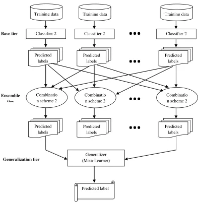
3 METHODOLOGY
Figure 3.1 Depiction of data processing at different tiers of MTSE
The dataset is splitted into 2 sets S1 & S2 at 80% & 20% proportionately. S1 is utilized for training and S2 is utilized for final testing. In base tier, 10-fold cross-validation is utilized to decrease the bias. The set S1 is divided into 10 sets of equivalent size. In every fold, 9 of these sets are combined and made use for training base models, and the left-out set is used for testing base models. This is rehashed for 10 folds by choosing an alternate set for testing. In this manner each set is utilized 9 times for training and once for testing. The outcomes in cross-validated predictions for every instance in S1. The ensemble tier uses the accompanying combination schemes.
Plural Voting Majority Voting
Weighted Majority Voting Confidence-Based Voting
Logistic Regression is utilized as meta-classifier in generalization tier. The basic features from the information space are chosen by considering their co-variance with class labels. The main three features with high co-variance values are chosen. The combination scheme predictions
alongside the chosen features structures the generalization tier input. Both SE & MTSE are tried with set S2. Models are compared by considering the accuracy. MTSE is superior than SE by the following 2 reasons,
Assume the predictions from every one of base classifiers as an irregular variable. The combination in ensemble tier is joint conveyance of these arbitrary factors. The joint dissemination takes all the pair-wise interaction of the irregular factors into thought. The various combination plans characterize numerous joint distributions of the arbitrary factors. Every one of these irregular factors is additionally a function which maps the input space to class labels. Because of this, combination scheme output gives highlights which not just exemplify the relationship among predictions from base tier and actual labels yet additionally the relationship among input space and class labels. These features give more quality data about input space than actual features in input space. Subsequently training the model on these features yields models with better precision. Contingent on misclassification paces of the base
classifiers, the predictions from every one of the Predicted label
Generalizer (Meta-Learner)
Training data
Classifier 2
Predicted labels
Combinatio n scheme 2
Predicted labels Training data
Classifier 2
Predicted labels
Combinatio n scheme 2
Predicted labels
Training data
Classifier 2
Predicted labels
Combinatio n scheme 2
Predicted labels
…
…
…
…
Base tier
Ensemble tier
base classifier contains False Positives (FP) set and False Negatives (FN) set. When suitable classifiers are utilized in base tier, every one of these sets becomes pretty much supplement to one another. With large pool of base classifiers, quantity of normal components between them will in general zero. When base classifiers differ for various sets of models, the combination plots in multi-tier guarantees that the shortcomings of the base classifier are made neutral with one another. Subsequently combination schemes produce better highlights. At the point when these features are trained utilizing a reasonable classifier, it sums up superior to SE.
Notwithstanding the above-expressed reasons, MTSE is appropriate for ample majority of classification issues because of the accompanying reasons moreover.
Statistical Reason: ensemble tier in MTSE consolidates the predictions of base classifiers utilizing distinctive combination schemes. This guarantees the insecurity of selecting an off-base classifier is diminished. The hazard is additionally diminished at generalization tier, as it sums up the outcome from various combination schemes. Computational Reason: MTSE totally dispenses
with the probability of finding the neighborhood optima. The decent variety in MTSE guarantees the better guess of the basic function between input information and class label.
Representational Reason: Even if every one of the base classifiers can't really speak to the fundamental function, combination scheme guarantees that space of the hidden function is extended. Generalization tier grows this space further. Henceforth MTSE can genuinely speak to the fundamental function.
i. Mathematical Model
Let be dataset, where and N is the complete number of occurrences in dataset and are class labels. Regularly, input space X comprises of numerous features and henceforth its components are represented by N-tuple of ‘d’ measurements.
where ‘d’ - quantity of features in input space. Thus, dataset is given as:
{( ) }
Split D into 2 sets S1 & S2 at 80% & 20% separately. S1 is utilized as training set & S2 is utilized as test set.
a. Base Tier
Let be set of weak classifiers. Let be the equal size sets, partitioned from the set .
Fold 1: Training set Testing set
Train the weak classifiers using T.
The weak classifiers maps the elements of T into one of classes in Y.
where and belongs to
In the next fold, is considered as testing set and remaining nine sets combined together are taken as training set. This is looped until every partitioned set in S1 are considered as testing sets. This results in the predictions for all the instances in T. Let be labels set predicted by weak classifiers.
Where
Algorithm 1: Base Classifiers Classification
Output: The labels (WL) predicted by the weak classifiers Randomly split D into 2 sets of size 80% and 20% and name
1 into ten sets of equal size 10% and name them as
⋃
Combine predictions of all ten folds of weak classifier into single set.
b. Ensemble Tier
Let be set of combination schemes and they combine the labels predicted by weak classifiers and map them into one of classes in Y.
( ( )) Where
Let be the set of labels predicted by the ensemble classifiers. This can be represented in mathematical form as
( ( ))
Where k = 1, 2, …, m
Output: labels (EL) predicted by ensemble classifiers
Corresponding to each class label, initialize a counter to
For each occurrence of a class label in classifier’s prediction, increment the corresponding counter
Class label corresponding to the Max_Count
Confidence-Based Voting:
For all instances, store the class probabilities of all the classifiers for all the classes into an array
_𝑃 𝑏← Max (class probabilities of every classifier for all the classes)
← The class label corresponding to Max_Prob End
Weighted Majority Voting:
Use Brute Force Algorithm for finding base learners optimal weights.
𝑏
Do for //Repeat for every weak classifier //Find sum of products of the weights ( ) and the class probabilities (𝑃 )
← + ∗𝑃
End End
Calculate Accuracy of ensemble classifier
c. Generalization Tier
This tier takes the top three critical features ensemble predictions EL and the actual labels Y as input. It produces the generalized predictions. This can be mathematically represented as
({ ( )})
is the generalization classifier or meta-learner and 𝐺 is final prediction produced by meta-learner. GC generalizes the labels predicted by ensemble classifiers into one of classes in Y.
Accuracy of Classification
Accuracy of classifiers is calculated using test set S2. The ratio between the counts of correctly classified instances to the total number of instances classified gives the accuracy.
𝑃
𝑃 𝑃 Where TP - #True Positives,
TN - #True Negatives, FP - #False Positives
FN - #False Negatives in the final prediction. As MTSE focuses on improving the TP and the TN, accuracy is only performance measure considered here.
Algorithm 3: Meta-learner Classification
Input: The labels (EL) predicted by the ensemble classifiers Output: The final labels (GL) predicted by the generalizer Calculate the covariance with a class label for each of the features in input space
// Used for picking the critical features
CF ←Pick three features with high covariance values Combine the critical features and the ensemble predictions TS ← CF EL
Train the generalizer with the set TS
Run the model obtained in step 6 with the set S2 Calculate accuracy of the generalizer
End
4 EXPERIMENTAL EVALUATION
These datasets are publicly available in the github.com, here political twitter dataset is considered. Initially in base tier, bias is reduced by multiple incremental learners with cross-validation which is shown in figure 4.1 where the incremental learners processes the incoming datastreams and produce the output by removing bias that is displayed in figure 4.2.
Figure 4.2: Removal of Bias
The combinations schemes and the meta-learners reduce the variance. Henceforth an ideal balance among bias and variance is accomplished. Thus, accuracy of classification improves. The ensemble tier uses the following combination schemes. Plural Voting (PV), Majority Voting (MV), Weighted Majority Voting (WMV).
Figure 4.3: Weight calculation
PV and MV use the cardinality to make the decision. WMV assigns weights based on incremental learner’s class probability which is shown in figure 4.3. By this the variance is reduced in this ensemble tier shown in figure 4.4. The generalization is done at final tier by Logistic Regression (LR).
Figure 4.4: Removal of Variance
Finally the opinion strength is calculated to analyze the dataset with positive and negative data using logistic regression that is done in the final generalization tier.
Figure 4.5: Opinion Strength Calculation
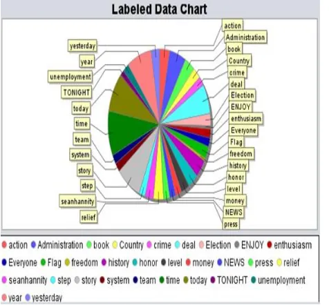
Below graph in figure 4.7 depicts the number of times the words repeated in the dataset. This helps to classify the positive and negative words.
Figure 4.7: Labeled chart of repeated words in dataset
The influence of introducing a new tier into SE was studied using the datasets and found the accuracy between SE & MTSE. This analysis is shown in figure 4.8. Overall, the performance of MTSE is superior to traditional SE algorithm.
Figure 4.8: Comparison of accuracy between MTSE & SE
5 CONCLUSION
This examination presented a MTSE algorithm by including another tier into the customary SE. The test results bring up that MTSE accomplished a superior accuracy than SE. From this investigation, it is transparent that the presentation of another tier into SE gives unrivaled execution for balanced/unbalanced datasets, datasets with high/low dimension and datasets with high/low volume. Henceforth we prescribe the utilization of MTSE for classification issues in real time domains. This examination can additionally be improved via doing feature engineering for datasets. This is required to improve the exhibition
further and consequently make MTSE the most dependable answer for classification issues. Furthermore, we are likewise investigating if MTSE is appropriate for incremental learning utilizing data streaming.
6 REFERENCES
[1] Ali, S., Tirumala, S. S., & Sarrafzadeh, A. (2015, July). Ensemble learning methods for decision making: status and future prospects. In 2015 International Conference on Machine Learning and Cybernetics (ICMLC) (Vol. 1, pp. 211-216). IEEE.
[2] Dietterich, T. G. (2000, June). Ensemble methods in machine learning. In International workshop on multiple classifier systems (pp. 1-15). Springer, Berlin, Heidelberg.
[3] Aldave, R., & Dussault, J. P. (2014). Systematic Ensemble Learning for Regression. arXiv preprint arXiv:1403.7267.
[4] Vilalta, R., & Drissi, Y. (2002). A perspective view and survey of meta-learning. Artificial intelligence review, 18(2), 77-95.
[5] Seewald, A. How to Make Stacking Better and Faster While Also Taking Care of an Unknown Weakness. Proceedings of the 19th International Conference on Machine Learning (2002).
[6] Liu, M., Zhang, D., Yap, P. T., & Shen, D. (2012, October). Hierarchical ensemble of multi-level classifiers for diagnosis of Alzheimer’s disease. In International Workshop on Machine Learning in Medical Imaging (pp. 27-35). Springer, Berlin, Heidelberg.
[7] Baumann, F., Ehlers, A., Vogt, K., & Rosenhahn, B. (2013, June). Cascaded random forest for fast object detection. In Scandinavian Conference on Image Analysis (pp. 131-142). Springer, Berlin, Heidelberg. [8] Ekbal, A., & Saha, S. (2013). Stacked ensemble coupled
with feature selection for biomedical entity extraction. Knowledge-Based Systems, 46, 22-32.
95 95.5 96 96.5 97 97.5 98 98.5 99 99.5 100
MTSE SE
A
cc
u
ra
cy