Physics of unstable nuclei: from structure to sequential decays
Alexander VolyaaDepartment of Physics, Florida State University, Tallahassee, Florida 32306-4350, USA.
Abstract. In this presentation we discuss features of nuclear structure and properties of nuclear decays that result from coupling to the reaction states with one and two nucleons in the continuum. Physics of the one-body decays is reviewed, and perturbations due to the virtual excitations into the continuum of reaction states are examined. The two-body decays are explored using the sequential decay mechanism. The two-neutron s-wave breakups are of particular interest, here the two-body nature of the process appears to suppress the decay rate as compared to the kinematically equivalent one-body s-wave decay. The effective phase space scaling and the resulting from it decay width as a function of the available energy are examined for identical and non-identical particles assuming different values of the scattering length.
1 Introduction
Experimental observations of multi-nucleon decays, such as the ones reported in Refs. [1–4], challenge our theoreti-cal understanding of the nuclear dynamics on the verge of stability. Tying together the nuclear many-body structure and physics of decay is not an easy task. Selected recent efforts in this direction can be found in Refs. [5–8]. In this contribution we discuss some generic aspects of particle decay, interplay between structure and reactions, and fea-tures of the three-body breakup.
2 One-body decay
2.1 Single particle decay amplitude
We assume that a one-body decay I1 → I2, illustrated in figure 1, proceeds due to an interaction component of the HamiltonianHQP1. In this process a resonant stateI1
emits a particle with energyϵ,and the system transitions into a final state I2 of the daughter nucleus. In the Fesh-bach projection formalism used in Refs. [6, 9] the compo-nentHQP1 is the one that connects the intrinsic spaceQ with the one-body continuum spaceP1.The external space P = P1+P2. . . where the subscript denotes the number of particles in reaction continuum. The decay amplitude is defined as
A1,2(ϵ)=⟨I2, ϵ|HQP1|I1⟩. (1)
a e-mail:[email protected]
1
2
Fig. 1.Illustration of the one-body decay processI1→I2.
TheI1→ϵ I2partial decay width, corresponding to this am-plitude, is given by the Fermi Golden Rule
dΓ1,2(ϵ)=2πA1,2(ϵ) 2
δ(E1−E2−ϵ)dϵ. (2)
The same result follows from the Feshbach projection for-malism, see Refs. [6, 9]. The total width is a function of the available energyϵ=E1−E2,
Γ1,2(ϵ)=2πA1,2(ϵ) 2
. (3)
The one-body continuum states|I2, ϵ⟩in the space P1are energy-delta-function normalized; therefore the amplitudes are normalized to include the density of states. Direct eval-uation of the overlap amplitude in Eq. (3) is a common method of evaluating the single particle decay width [10]. If the one-body HamiltonianHQP1is given by a spherically
symmetric potentialV(r) then the amplitude in Eq. (1) is
A1,2(ϵ)= √
2µ π~2k
∫ ∞
0
dr uI1(r)V(r)FI2(kr). (4)
Herek= √2µϵ; the initial stateI1is described by a single-particle radial wave function uI1(r); the final state in the continuum is given by the Coulomb (Bessel) functionFI2(kr); and the coefficient in front of the integral reflects the energy-delta-function normalization of states in the continuum. At low energies the energy-dependence of the amplitude is determined by the asymptotic of the function FI2(kr) as kr→0.In this limit the dependence of the decay width on energy is commonly expressed using the phenomenologi-cal R-matrix formalism [11] via sphenomenologi-calingχand the channel radius parameterR:
Γ(ϵ)≃2χγw(R)P(kR), (5)
where
P(kR)= kR
F2(kR)+G2(kR) and γw(R)= 3~2 2µR2. (6)
HereGis the irregular Coulomb (Bessel) function. In this work we discuss neutral particles, in which caseP0(x)=x
DOI: 10.1051/
C
Owned by the authors, published by EDP Sciences, 2012
epjconf 20123/ 803003
This is an Open Access article distributed under the terms of the Creative Commons Attribution License 2 0 , which . permits unrestricted use, distributi and reproduction in any medium, provided the original work is properly cited.
0.01 0.1 1 10 10
-7 10
-6 10
-5 10
-4 10
-3 10
-2 10
-1 10
0 10
1
0p
0d 5/2 0d
3/2
[
M
e
V
]
[MeV] 1s
1/2
Γ
Fig. 2.Energy dependence of the single-particle decay widths for neutral particles. Thin straight lines show the power-law scaling
Γ∝ϵβwhereβ=l+1/2,as follows from Eq. (5) in theϵ →0
limit; solid lines represent calculations with Eq. (4). Experimen-tal points are marked for5He (ϵ=0.895 MeV,Γ=648 keV),17O (ϵ =0.941 MeV,Γ =98 keV), and19O (ϵ=1.540 MeV,Γ =310 keV), see Ref. [6].
andP1(x) = x3/(1+x2),in generalPl(x) ∝ x2l+1 when x≪l+1/2.The dependence of the single-particle decay width on energy is shown in figure 2. At high energies the amplitude goes to zero and the treatment is analogous to Born approximation.
2.2 Interaction with one-body continuum
The coupling to the continuum amounts to an additional effective interaction Hamiltonian [6, 9] in the internal space Q,
H′(ϵ)= ∫ ∞
0
dϵ′ |A(ϵ
′)|2
ϵ−ϵ′+i0. (7)
Here, we assume an on-shell form which emerges when the internal and continuum spaces are orthogonal; the general expression and its derivation can be found in Ref. [6, 9]. In the single channel example for brevity of notations the subscripts are omitted,A1,2 ≡A,and all energies are mea-sured form the channel’s thresholdE =ϵ.The interaction in Eq. (7) is analogous to the second order energy perturba-tion due to excitaperturba-tions into the continuum. The Feshbach projection formalism, however, is exact; the exact eigen-values in the full space are found from an energy depen-dent HamiltonianH(E) = HQQ +H′(E) using the non-linear version of Schroedinger’s equationH(E)|I⟩=E|I⟩. In generalH′ andH are non-Hermitian. If for some de-cay channel ϵ > 0 then the integration region in Eq. (7) contains a pole and the integral can be separated into the Hermitian principal value part∆(ϵ) (self-energy) and the remaining non-Hermitian termΓ(ϵ) (the decay width):
H′(ϵ)=∆(ϵ)− i 2Γ(ϵ),
where
∆(ϵ)=− ∫
dϵ′ |A(ϵ
′)|2
ϵ−ϵ′+i0, Γ(ϵ)=2π|A(ϵ)|
2.
The real and imaginary parts ofH′are shown in figure 3 for17O. In this example we assume an intrinsic state in the space Qto have a harmonic oscillator wave function, the oscillator frequency beingω=41A−1/3MeV.The cou-pling to continuumHQP1in Eq. (4) is modeled by a Woods-Saxon potential. It was found that for both s- and d-waves the amplitude at low energies is well parameterized by Eq. (5) withχ=0.256 andR=4.81 fm.
The role of the non-Hermitian part Γ in the nuclear many-body problem is discussed in Refs. [6, 9]. This term has a factorized form, which maintains the unitarity of the scattering matrix. The factorized form leads to a dynami-cal phase transition [12], also known as superradiance [13]. The Hermitian correction from virtual excitations into the continuum, ∆(ϵ), modifies positions of bound and reso-nant states near decay thresholds. Sharp changes in spec-troscopic observables near thresholds have been studied in Ref. [14]. The strongest, cusp-like effect is seen in figure 3 for the s-wave,∆0(0) =−1.2 MeV. For other angular mo-mentum channels the magnitude of∆(ϵ) is smaller and its energy behavior is more continuous. The importance of the self-energy term in near-dripline nuclei is discussed in Ref. [9]. The subject, however, is far from being settled. First, most successful effective shell model interactions are ad-justed to experimental observables and therefore include the self-energy in some averaged form. Second, the phe-nomenological shell model implies some mean-field single-particle basis with wave functions that are more realistic than those of the harmonic oscillator examined figure 3, therefore the resulting self-energy corrections are small. Moreover, the stationary bound states of a given mean field potential, such as solutions of the Woods-Saxon potential, are eigenstates which are not subject to any additional per-turbation due to the one-body continuum.
3 Two-body decay
3.1 Sequential decay
In this section we continue the discussion in Ref. [6] fo-cusing on selected aspects of the two-body decay, related studies can be found in Ref. [15]. Here a system is coupled to states involving more than one particle in the continuum. The two-body decay represents a transition fromQtoP2. This can be generated by a direct three-body interaction HamiltonianHQP2or by a second order sequential process
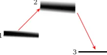
involving HQP1.We examine the second case, referred to as the sequential decayI1 →ϵ1 I2 →ϵ2 I3,see illustration in figure 4. A somewhat analogous process takes place in the two-photon decay from the 2s state in the Hydrogen atom. The amplitude for the two-body decayI1→ϵ1 I2→ϵ2 I3is
A1,2,3(ϵ1, ϵ2)=
A1(ϵ1)A2(ϵ2) ϵ2−
(
E2−2iΓ2,3(ϵ2)
). (8)
Here we present an on-shell formE1 =ϵ1+ϵ2+E3; we also assume that the width of the intermediate state is fully
determined by the single decay channelI2 →ϵ2 I3; and, fi-nally, we set the energy scale so that E3 = 0.The Fermi Golden Rule gives the partial decay width distribution for the sequential process as
dΓ(E) dϵ1dϵ2 =
0 0.5 1 1.5 2 2.5 3 3.5 4 4.5 5
-20 -15 -10 -5 0 5 10 15 20
Γ
[MeV]
ε
[MeV]
-3 -2.5 -2 -1.5 -1 -0.5 0 0.5 1 1.5 2
∆
[MeV]
s-wave d-wave
Fig. 3.Example of corrections due to the one-body continuum in 17O. Self-energy∆(ϵ) and widthΓ(ϵ) are shown as functions of
energyϵmeasured from the threshold.
1
2
3
Fig. 4.Illustration of the sequential decay processI1
ϵ1
→I2
ϵ2
→I3.
The total amplitudeAT in Eq. (9) must include amplitudes for all intermediate states, and it should be (anti) sym-metrized for identical particles.
WhenE2 > E1,this case is illustrated in figure 4, the intermediate state is higher in energy which creates an en-ergy barrier for the decay. The traditional sequential pro-cess occurs whenE2 < E1and the direct one-body decay channel is open leading to an emission of the first parti-cle with energyϵ1 = E1−E2.In this case the amplitude (8) has a pole at this energy (at the poleE2 = ϵ2). If an intermediate state is narrow one can use the following ap-proximationΓ/|E−iΓ/2|2 ≈2πδ(E).This approximation leads to the classically expected result that the lifetime of the initial state is fully determined by the first step in the sequential decayI1→ϵ1 I2,thereforeΓ1,2,3=Γ1,2.
In figure 5 the integrated two-body sequential decay width is shown as a function ofE2 in the case when both particles are emitted in thed-wave. It is assumed thatE1= 1 MeV (E3 = 0). While E2 < E1 and the direct single-particle decay channel is open Γ1,2,3 ≃ Γ1,2. In figure 5 the one-body widthΓ1,2 (blue dashed line) coincides with Γ1,2,3 (red solid line) in this limit. At energiesE2 > E1,
0.0 0.5 1.0 1.5 2.0
10-4
0.001 0.01 0.1 1
E2@MeVD G1,2,3
@
MeV
D
Fig. 5. Sequential d-wave two-nucleon decay width Γ1,2,3 is shown as a function of the intermediate state’s energy E2 (red line). The initial state is at energyE1=1 MeV; the final state is atE3=0 MeV. The single-particle decay width is assumed to be
Γ1,2(ϵ)=Γ2,3(ϵ)=0.3158ϵ5/2(ϵandΓare in units of MeV). The
Γ1,2(E1−E2) is shown with dashed-blue line.
0
2
4
6
8
0.1
0.2
0.5
1.0
2.0
5.0
E
2@
MeV
D
G
1,2,3@
MeV
D
Fig. 6. Same as in Fig. 5 but assuming an s-wave process. The single-particle decay width is parameterized as Γ1,2(ϵ) =
Γ2,3(ϵ)=7.0
√
ϵ(ϵandΓare in units of MeV).
the sequential decay proceeds via a virtual resonant state, while the direct one-body decay is no longer possible.
In the case when both neutrons are emitted in the s -wave, figure 6, the narrow width approximation is no longer valid. It may be counterintuitive, but, as seen from figure 6, the condition Γ1,2,3 = Γ1,2,expected classically for a sequential process, is not fulfilled. Due to the extremely short-lived nature of an intermediate state it is appropri-ate to interpret the process as a three-body breakup rather than as sequential. It is interesting that the lifetime of the initial stateI1becomes longer if its daughter product, the state I2,is unstable to further s-wave decayI2 → I3.For E2 <1 MeV in figure 6 the sequential decay widthΓ1,2,3 (in solid red) is smaller thanΓ1,2(in dashed-blue). Narrow three-body s-wave states have also been discussed in Ref. [16].
3.2 Low energy s-wave decay
In this section we concentrate on the s-wave three-body breakup. We assume the one-body decay width to be given by Eq. 5 withχ =2/3, see Ref. [17], andΓ1(ϵ) = 2~
2
µ1R1k,
which is proportional to √ϵ, is the leading term in the de-nominator of Eq. (8), thus the form of the scattering ampli-tude in the effective range expansion is recovered [18],
ϵ2− (
E2− i 2Γ2(ϵ2)
) ≈µ~2
2R2( 1 a2 +ik2).
This transfers the sequential picture of decay that takes place through a resonant state into a three-body breakup where an intermediate structure is described by the low-energy s-wave behavior. This behavior is controlled by the scattering lengtha2or equivalently with the energy param-eterε2:
a2≡ Γ2(ϵ) 2k E2
=µ ~2 2R2E2
, ε2≡ ~ 2
2m2a22
. (10)
In the following using Eq. (10) we substituteE2 with the virtual state energyε2 which, being tied to the scattering length, is a universal property of the s-wave scattering at low energies. As a result of this substitution for distinct particles, where the total amplitude is given by Eq.(8), we obtain
dΓ1,2,3(ϵ1ϵ2) dϵ′ =
2λ π
√
(E1−ϵ2)ϵ2 ε2+ϵ2 .
(11)
Here
λ=R2 R1
√µ 2 µ1
(12)
is a dimensionless parameter that is expected to be close to unity. The integrated decay width as a function of the resonance energyE1is
Γ1,2,3(E1)=λ [
2ε2+E1−2 √
ε2(E1+ε2) ]
. (13)
The phase space volume is an important factor in a re-action rate; at low energies it leads to a power lawΓ(E)∝ Eβ, see also Refs. [6, 8]. Let us examine the value of the scaling parameterβfor different processes. The one-body phase space leads toβ= 1/2 for the s-wave (symmetric) decay. The three-body phase space scales with energy with β=2 since∫ d3k
1d3k2δ(E−ϵ1−ϵ2)∝E2; and indeed at very low energies whenE1≪ε2we find from Eq. (13)
Γ1,2,3(E1)≃λ E2
1 4ε2
. (14)
In the other limitE1 ≫ε2,at higher energies or when the scattering length is large compared to the particle’s wave length at the decay energy,
Γ1,2,3(E1)≃λE1, (15)
andβ =1.This confirms that the decay is different from sequential because the scaling law is not that ofβ=1/2.
For identical particles the total amplitude isA±T(ϵ1, ϵ2)= [
A1,2,3(ϵ1, ϵ2)±A1,2,3(ϵ2, ϵ1) ]/√
2. The limit where E1 ≫ ε2is similar and corresponds toβ=1,
Γ±
1,2,3(E1)≃ π±2
π λE1. (16)
At low energies,E1 ≪ε2,the symmetric amplitude again leads toβ=2,
Γ+
1,2,3(E1)≃λ E21
2ε2
; (17)
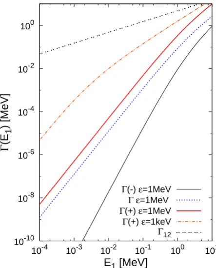
10-10 10-8 10-6 10-4 10-2 100
10-4 10-3 10-2 10-1 100 101
Γ
(E
1
) [MeV]
E
1[MeV]
Γ(-) ε=1MeV Γε=1MeV Γ(+) ε=1MeV Γ(+) ε=1keV Γ12
Fig. 7.Γ1±,2,3(E1) (labeled asΓ(+) andΓ(−)) and Γ1,2,3(E1) for distinguishable particles (labeled asΓ) are shown as functions of the total decay energy E1. The values of ε2 are indicated. The one-body decay width Γ1,2(E1) as a function of energy is also shown.
however, the destructive interference of terms in the anti-symmetric amplitude results inβ=3 inE1 ≪ε2limit,
Γ−
1,2,3(E1)≃ 3π−8
24π λ E3
1 ε2 2
. (18)
In figure 7 the quantityΓ1,2,3(E1) is shown as a function of E1for these cases. The one-bodyΓ12(E1) is also included to highlight a relatively long-lived nature of configurations involving two s-wave neutrons. The finding appears to sup-port ideas in Ref. [16]. It is remarkable that the predicted s-wave two-body decay width in the experimentally-relevant region of energy appears to follow a simple law Γ ≃ E. The changes in the phase-space energy scaling considered in this work emerge due to quantum evolution via an inter-mediate-state; similar discussions can be found in Refs. [1, 16, 19, 20].
This work is supported by the U.S. DOE grant DE-FG02-92ER40750.
References
1. A. Spyrou, Z. Kohley, T. Baumann, D. Bazin, B. A. Brown, G. Christian, P.A. DeYoung, J.E. Finck, N. Frank, E. Lunderberget al., Phys. Rev. Lett.108, 102501 (2012)
3. E. Lunderberg, P.A. DeYoung, Z. Kohley, H. At-tanayake, T. Baumann, D. Bazin, G. Christian, D. Di-varatne, S.M. Grimes, A. Haagsmaet al., Phys. Rev. Lett.108, 142503 (2012)
4. H.T. Johansson, Y. Aksyutina, T. Aumann, K. Boret-zky, M.J.G. Borge, A. Chatillon, L.V. Chulkov, D. Cortina-Gil, U.D. Pramanik, H. Emlinget al., Nucl. Phys.A847(2010)
5. N. Michel, W. Nazarewicz, M. Ploszajczak, and J. Okolowicz, Phys. Rev. C67, 054311 (2003) 6. A. Volya and V. Zelevinsky, Phys. Rev. C74, 064314
(2006)
7. T. Myo, K. Kato, and K. Ikeda, Phys. Rev. C 76, 054309 (2007)
8. L.V. Grigorenko, I.G. Mukha, C. Scheidenberger, and M.V. Zhukov, Phys. Rev. C84, 021303 (2011) 9. A. Volya, Phys. Rev. C79, 044308 (2009)
10. S. Åberg, P.B. Semmes, and W. Nazarewics, Phys. Rev. C56, 1762 (1997)
11. D. Baye and P. Descouvemont, Rep. Prog. Phys.73, 036301 (2010)
12. I. Rotter, J. Phys. A42, 153001 (2009)
13. N. Auerbach and V. Zelevinsky, Rep. Prog. Phys.74, 106301 (2011)
14. N. Michel, W. Nazarewicz, M. Ploszajczak, and T. Vertse, J. Phys. G36, 013101 (2009)
15. J. Rotureau, J. Okolowicz, and M. Ploszajczak, Nucl. Phys.A767, 13 (2006)
16. L.V. Grigorenko and M.V. Zhukov, Phys. Rev. C77, 034611 (2008)
17. A. Bohr and B.R. Mottelson, Nuclear Structure (World Scientific Publishing, 1998)
18. L.D. Landau and E.M. Lifshitz,Quantum mechanics. Non-relativistic theory.(Pergamon Press, New York, 1981)
19. Steven E. Koonin, Phys. Lett. B70, 43 (1977) 20. R. Lednicky and V.L. Lyuboshits, Sov. J. Nucl. Phys.