A New Pooling Method For Improvement Of
Generalization Ability In Deep Convolutional
Neural Networks
El houssaine HSSAYNI , Mohamed ETTAOUILAbstract: As powerful visual models, deep learning models, in particular, deep convolutional neural networks(DCNNs) have demonstrated remarkable performance in various challenging artificial intelligence and machine learning tasks and attracted considerable interests in recent years. A pooling process plays a very important role in deep convolutional neural networks, which serves to reduce the dimensionality of processed data for decreasing computational cost as well as for avoiding overfitting and improving the generalization capability of the network. Although standard pooling techniques, such as the max pooling and the 𝑙 pooling (where 𝑝 ≥ 1 ) are typically adopted in various studies, we alternatively propose, in this paper, a new pooling method named 𝑙 pooling in order to improve the generalization capability of DCNNs. Experimental results on two image benchmarks indicate
that 𝑙 pooling outperforms the existing pooling techniques in classification performance as well as is efficient for enhancing the generalization
capability of DCNNs. Moreover, we show that the 𝑙 pooling combined with other regularization methods, such as dropout and batch normalization, is
competitive with other existing strategies in classification performance.
Index Terms: Convolutional Neural Networks, Deep Neural Networks, Generalization Ability, 𝑙 Regularization, Pooling methods, Regularization
methods.
————————————————————
1
INTRODUCTION
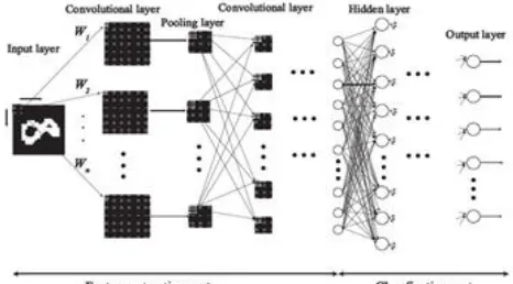
Nowadays, deep learning models have evolved rapidly and attracted a great deal of attention due to their crucial success in various areas, such as image recognition, object detection, speech recognition, and many other domains such as genomics and drug discovery. Its outstanding and high capability to learn very complex relationships directly from the data makes deep learning models perfectly appropriate to carry out intelligent tasks successfully, similar to those achieved by the human brain. There are many deep neural network architectures [1] such as deep Boltzmann machine, deep belief network, and deep convolutional neural networks. Recently, Deep Convolutional neural network (DCNN), one of the popular and powerful deep neural networks which initially presented for computer vision task [2], has constantly shown hopeful results and significant improvement in various fields and applications, including image recognition [3], speech recognition [4], time series forecasting [5], etc. This improvement and high performance are achieved because of their one of kind qualities such as weight sharing, localized sparse neuronal connectivity, and consolidated utilization of two distinct sorts of layers. The Convolutional Neural Network is an extraordinary class of multilayer feedforward neural systems, which imitates a neurobiological process in the animal visual cortex and empowers to deal with crude images legitimately without preprocessing. Generally, CNN is composed of two parts: the feature extraction part and the classification part (as shown in Fig.1).
The feature extraction part receives in input an image pattern to be processed and transforms it into a set of smaller images (called feature maps) representing the local features of the input image. It is primarily formed by a sequence of convolutional layers and pooling (subsampling) layers. The convolutional layer aims to extract the patterns, found within local regions of input maps, by applying many filters to the inputs, computing the convolution product of every filter and inputs, then convolutional layer’s output is obtained by applying a non-linear function of the convolution operation’s output. The resulting activations are then passed to the pooling layer, which means to accomplish spatial invariance by lessening the resolution of feature maps, for enhancing the computational efficiency of CNNs. The second part of CNN (the classification part) is formed by a standard multilayer perceptron which receives in input the features extracted in the first part and outputs a probability for each class label. In this paper, we focus on the feature extraction part and especially on the pooling layer, which plays a crucial role in CNNs since it is essentially responsible for the invariance to data variation and perturbation [6]. The inspiration driving pooling is that activations in the pooled map are less delicate to the precise locations of structures inside the image than the original feature map [2]. The pooling layer is acquired by applying a pooling mechanism to assemble information inside each small region of the input feature maps and then down sampling the results [7]. Some past studies have concentrated on pooling strategies that intend to accomplish spatial invariance by lessening the resolution of feature maps, for enhancing the computational efficiency of CNNs, and obtain large increases in performance. As well as reducing the overfitting problem. The most standard and popular pooling technique is the max pooling [8], which features just the maximum activations in the pooling region by evacuating background information. Be that as it may, it likely leads to overfitting problem in practice [9]. The second most popular pooling method is the average pooling [10], which considers uniformly all the activations in the pooling region, and takes the arithmetic mean of the elements in each pooling region. Be that as it may, when joined with the widely used rectified linear
_______________________________
• El houssaine HSSAYNI, is a Ph.D. student in the Laboratory of Modeling and Mathematical Strictures at the Faculty of Sciences and Techniques, University Sidi Mohamed Ben Abdellah of Fez, Morocco. he works on Deep Neural Networks, regularization problems, statistical learning methods and applications. E-mail : [email protected]
40 unit (ReLU) activation function, it can take many zero
activations into account and down weight strong activations [9]. In order to overcome these downsides, various modified pooling techniques have been proposed. Examples of such methods include stochastic pooling method [9] which considers a probability distribution of the pooling region activations and from this distribution takes a randomly sampled activation as an output. It demonstrates a better generalization capability than those with the average and the max pooling for some benchmark datasets. The hybrid pooling method [11] randomly picks the average pooling or the max pooling in each pooling layer. The pooling strategy for each convolutional feature map is stochastically picked with a certain probability. In image classification tasks with benchmark datasets, the hybrid pooling method shows an effective increasing of the generalization capability of CNNs. A successful variant of pooling methods is 𝑙 pooling [12], which calculates the output of the pooling region using an 𝑙 norm with a real value 𝑝 ≥ 1, and can be regarded as a generalized deterministic pooling method including both the average pooling (for 𝑝 1) and the max pooling (for 𝑝 ) as special cases. Moreover, by inspiring to the regularization theory, which affirm that an 𝑙 regularization method produces a sparse solution only when ( 𝑝 1), and the smaller the 𝑝, the sparser the solution [13], and according to the work [14], we propose a novel polling method named 𝑙 pooling, which use the absolutely homogeneous
function to calculate the output of the pooling region. To further justify our proposed method, we conduct several experiments on two benchmark image datasets: the MNIST dataset [2] and the Fashion MNIST dataset [15]. The experimental results illustrate that 𝑙 pooling beats the
current pooling strategies in classification performance as well as is effective for enhancing the generalization capability of CNNs.
In summary, the main contributions of this paper are as follows:
• We propose a new simple, yet effective pooling method named 𝑙 pooling in order to improve the generalization
capability of DCNNs.
• We validate and demonstrate the performance of our proposed method on two public object recognition benchmarks.
• By combining the proposed method and other regularization methods, such as dropout and batch normalization, we have achieved the state-of-the-art classification performance with moderate parameters on two public object recognition benchmarks.
The reminder of this paper is organized as follows. In section 2 we present some deep neural networks regularization techniques. in Section 3 we give a description in detail about pooling process used in CNNs and briefly review the existing pooling methods. In section 4 we give a description in detail about our proposed method. In section 5, the effectiveness of 𝑙 pooling is shown in the numerical experiments on image
classification tasks with two benchmark image datasets. Moreover, the combination of 𝑙 pooling and other
regularization methods, such as dropout and batch normalization, is tested to show its high generalization capability. Section 6 covers the summary of our work.
Figure. 1. A standard Convolutional Neural Network
Architecture
2
REGULARIZATION
IN
DEEP
NEURAL
NETWORKS
In order to avoid overfitting, as well as to improve the generalization capability of Deep Neural Networks, various regularization techniques have been proposed, such as Dropout [2], DropConnect [16], and Batch Normalization [17].
2.1 Dropout
Dropout [2] is arguably the most popular strategy to avoid overfitting in deep neural networks. The random dropout layer generates a binary mask 1 , where each element of the mask is independently sampled from a Bernoulli distribution with a probability 𝑝:
This mask is used to obtain the output activations:
(2)
where, denotes the Hadamard product, and
denote the activations and biases respectively, is the weight matrix and is the activation
function.
2.2 DropConnect
DropConnect [16] is a generalization of the dropout technique where a randomly selected subset of weights in the network is set to zero. DropConnect is like Dropout as it presents dynamic sparsity inside the network, yet, contrasts in that the sparsity is on the network parameters , instead of the output vectors of a layer, therefore:
(3)
Where is a binary matrix encoding the connection information and defined as:
𝑙𝑙 𝑝 (4)
2.3 Data Augmentation
Data Augmentation [3] is another popular technique largely used to improve the training of convolutional neural networks. It consists to artificially enlarge the dataset using label-preserving transformations. Data augmentation verifiably regularizes the models and enhances generalization ability, as established by statistical learning theory.
2.4 Batch Normalization
Batch normalization [17] significantly reduces training time and enhances the generalization ability by reducing Internal Covariate Shift, by normalizing the input of each neural layer in the network. This technique draws its quality from making standardization a piece of the model design and playing out the standardization for each training mini-batch. Using batch normalization requires a few changes in accordance with the hyperparameters. The more noteworthy changes are:
Increment the learning rate: the standardization balances out the preparation procedure, permitting higher learning rates.
Expel dropout or use lower dropout rates: batch normalization additionally has a regularization impact. This impact decreases the requirement for dropout to the point it is not, at this point required. On the off chance that it is utilized, it ought to be utilized with lower rates.
Batch normalization has shown that is viable for expanding the speculation capacity of CNNs, as well as for avoiding overfitting problem.
3.
POOLING
MECHANISM
Pooling is a vital component in CNN which serves to avoid overfitting, as well as to acquire enormous increments in performance. The inspiration driving pooling mechanism is that enactments in the pooled map are less delicate to the exact areas of structures inside the image than the first component map [2]. A convolutional feature map is composed of a set of activations and a pooling operation is iterated for each subset of the feature map, named a pooling region. The pooling technique is a significant procedure in CNNs for removing important highlights in a given feature map. The pooling technique serves to decide an output of a pooling region for 1 , where a set of activations in is represented as | | where | | denotes the number of activations within the pooling region . Then the pooling feature map is obtained by collecting the outputs of all the pooling regions. In the remainder of this section, we briefly survey the existing pooling strategies.
3.1 Max Pooling
Max Pooling [8] is the most popular pooling method, which takes the largest activation in the pooling region as given in Eq.5.
1 (5)
Max Pooling is aimed for extracting local features such as lines, edges, and textures in the feature map.
3.2 Average Pooling
Average Pooling [10] takes the arithmetic mean value of activations in the pooling region as given in Eq.6.
1
| | ∑
1 (6)
This method can extract global features in a given feature map by smoothing the pooling region.
3.3 Stochastic Pooling
Stochastic Pooling [9] is an improved pooling strategy, which takes the activations inside each pooling region based on the
normalized probability distribution of activation values. In the training phase, it initially relegates a probability to every component in the pooling region as given in Eq.7.
𝑝
∑ 1 | |
(7)
Then the output of each pooling region is given by randomly sampling from a multinomial distribution with the probability parameter 𝑝 for 1 | | as follows:
𝑙 𝑝 𝑝| | (8)
In the testing phase, instead of the normal averaging, the probabilistic form of averaging is adopted, as given in Eq.9.
∑ 𝑝
1 (9)
This method is less prone to overfitting due to the stochastic strategy used, and outperforms the max and average pooling [10].
3.4 Hybrid Pooling
Hybrid Pooling [11] is another improved pooling strategy, which introduces a probability to choose the average or the max pooling technique for each convolutional feature map, where the chosen pooling strategies are utilized for all the pooling regions. In the training phase, for each feature map in the convolutional layer, the max pooling is used with probability 1 𝑝 and the average pooling with probability 𝑝 for all the pooling regions:
{
1
(10)
Where with
| |∑ 1
and with
In the testing phase, the output for each pooling region is given by the expected value of in Eq.10, which is given as follows:
𝑝 1 𝑝 (11)
This method has shown that is effective for increasing the generalization capability of CNNs.
3.5 𝒍 Pooling
𝑙 Pooling [12] is a successful variant of pooling which can be observed as a continuous parametrization transition from average pooling to max pooling. This method is a pooling method using the 𝑝 norm with a real value 𝑝 ≥ 1, defined as follows:
1
| |( ∑
)
1 (12)
42 large enhancements in error rate in computer vision tasks
compared to max pooling [12].
4.
PROPOSED
METHOD:
𝒍
𝟏 𝟐POOLING
In order to improve the generalization ability of deep CNNs as well as to avoid overfitting problem on the one hand, and due to the crucial role of pooling mechanism in the CNN and the successful of 𝑙 pooling method on the second hand, and by inspiring to the regularization theory, which affirms that an 𝑙 regularization method produces a sparse solution only when ( 𝑝 1), and the smaller the 𝑝, the sparser the solution [13], and according to the work [14], we propose a novel polling method named 𝑙 pooling, which uses the absolutely
homogeneous function to calculate the output of the pooling region.
This pooling method serve to determine the output of the pooling region for 𝟏 as follows:
1
| |( ∑ √| |
) 1 (13)
Where and | | are defined as in the previous section.
5.
EXPERIMENTS
RESULTS
To justify the effectiveness of our proposed method, we conduct several experiments on two popular benchmark image datasets: the MNIST dataset [2] and the Fashion-MNIST dataset [15]. The structures of these datasets are described below.
5.1 Used dataset
The MNIST (Modified National Institute of Standards and Technology) [2] is a standard and widely adopted dataset for classification tasks on handwritten digits. It is composed totally of images, among which images are used for training and the remaining 1 images for testing. All images consisting of pixels, each of which has pixel values corresponding to grayscale color intensities. Basically, the task is to classify the images into 1 digit classes MNIST constitute a baseline of the validation for most deep learning approaches and here we first perform experiments on MNIST to make a basic verification of our proposed method. The Fashion-MNIST is a novel image dataset, recently proposed by [15] which is intended to serve as a direct drop-in replacement for the original MNIST dataset. The Fashion-MNIST dataset has all the characteristic of the original MNIST’s, which is composed of 28x28 pixel of grayscale fashion thumbnail images with 60,000 training and 10,000 test samples. The task is to classify the images into 10 categories of fashion products. Figure.2 shows class names and example images in Fashion-MNIST dataset.
Figure. 2. Class names and example images in
Fashion-MNIST dataset.
5.2 Simulation methods
We performed numerical experiments utilizing the deep learning framework Caffe [12]. The Rectified Linear Unit (ReLU) was used as the activation function for both the fully connected and convolution layers. The softmax function was utilised as the activation function for the last layer (output). Our neural network was trained utilizing the mini-batch stochastic gradient descent method, such as the size of each batch is 128. The momentum was set at (the momentum is the weight of the last gradient update), the coefficient of weight decay (i.e. the coefficient of the regularization term integrated in the loss function) and the coefficient of bias decay was set at . In the initialization phase, we have initialized the weights between all the layers by randomly sampled from a Gaussian distribution with mean zero, and the standard deviation was set at 0,0001 for the first convolutional layer, 0,01 for the rest convolutional layers, and 0,1 for the fully connected layers. The biases in the initialization phase were set at 0 for all the layers. For all the convolutional operations, the convolutional kernel size is and the stride is 1. For all the pooling operations, the pooling region size is and the stride is 2. The learning rate for the weight update was set at 0,01 for the initial 130 cycles, at 0,001 for the following 40 emphases, and at 0,0001 for the last 20 emphases.
5.3 Numerical results and discussion
We performed numerical experiments on image classification tasks to verify the effectiveness of our proposed method. We compare Training time and Prediction accuracy of the network using each of pooling methods: first we use Max poling as a pooling method used in the pooling layers, after, we use Average pooling, then we use our proposed 𝑙 Pooling and
finally we combine our proposed pooling method with a regularization technic: for MNIST we have used Dropout for enhance the generalization ability of the network, and for Fashion-MNIST we have combined 𝑙 Pooling with Batch
normalization in order to achieve better performance.
Table 1: Training time (S) and classification accuracies (%) on MNIST dataset.
Method Prediction accuracy Training time
Max Pooling 90.09 75.7
Average Pooling 90.18 75.16
l1/2 Pooling 92.16 75.11
l1/2 Pooling +
Dropout
93.24 78.52
As reported in Table 1, we observe that 𝑙 pooling achieves
a high prediction accuracy of 1 on the MNIST dataset. And when it combined with Batch Normalization, it achieves a high prediction accuracy of with a marginal increase in training time. For the Fashion-MNIST dataset, the obtained results are presented in the following table (Table 2):
Table 2: Training time (S) and classification accuracies (%) on
Fashion-MNIST dataset.
Method Prediction accuracy Training time
Max Pooling 88.72 164.7
Average Pooling 88.34 164.16
l1/2 Pooling 90.16 164.23
l1/2 Pooling +
Batch Normalization
91.57 167.52
As reported in Table 2, we observe that 𝑙 pooling achieves
a high prediction accuracy of 1 on the Fashion-MNIST dataset. And when it combined with Batch Normalization, it achieves a high prediction accuracy of 1 with a marginal increase in training time. The experimental results illustrate that the proposed method outperforms the existing pooling methods such as max pooling and average pooling in classification performance.
6.
CONCLUSION
Due to the crucial role of pooling mechanism in the CNN on the one hand, and the effectiveness due to the previously proposed 𝑙 pooling method (for 𝑝 ≥ 1) for enhancing the generalization ability of Deep Convolutional Neural Networks, on the other hand, we have alternatively proposed in this paper a new pooling method called 𝑙 pooling method which
uses the absolutely homogeneous function to calculate the output of the pooling region. Then Experimental results show that the proposed 𝑙 pooling method is superior to
some existing pooling methods on a range of datasets. As we have mentioned in Section 2, there have been various techniques for enhancing the generalization capability of the CNNs. These methods can be combined to further improve the generalization capacity if they are applied to different parts of the CNN. The proposed 𝑙 pooling has been combined
with the Dropout and the Batch normalization method in this work, but it can be combined with many other existing methods as well. Although we have shown the efficiency of the 𝑙 pooling using two benchmark image datasets: MNIST and
Fashion-MNIST, it would be significant to further verify it in other benchmark image datasets, as well as in other application tasks such as medical image recognition and time series forecasting.
REFERENCES
[1]. W. Liu, Z. Wang, X. Liu, N. Zeng, Y. Liu, and F. E. Alsaadi, ―A survey of deep neural network architectures and their applications,‖ Neurocomputing, vol. 234, pp. 11–26, 2017. [2]. Y. LeCun, L. Bottou, Y. Bengio, and P. Haffner,
―Gradient-based learning applied to document recognition,‖ Proceedings of the IEEE, vol. 86, no. 11, pp. 2278–2324, 1998.
[3]. Krizhevsky, I. Sutskever, and G. E. Hinton, ―ImageNet classification with deep convolutional neural networks,‖ in Advances in neural information processing systems, 2012, pp. 1097–1105.
[4]. G. E. Dahl, D. Yu, L. Deng, and A. Acero, ―Context-dependent pre-trained deep neural networks for large-vocabulary speech recognition,‖ IEEE Transactions on audio, speech, and language processing, vol. 20, no. 1, pp. 30–42, 2011.
[5]. W. Chen and K. Shi, ―A deep learning framework for time series classification using relative position matrix and convolutional neural network,‖ Neurocomputing, vol. 359, pp. 384–394, 2019. [6]. D. Scherer, A. Muller, and S. Behnke, ―Evaluation
of pooling operations in convolutional architectures for object recognition,‖ in¨ International conference on artificial neural networks. Springer, 2010, pp. 92–101.
[7]. M. Sun, Z. Song, X. Jiang, J. Pan, and Y. Pang, ―Learning pooling for convolutional neural network,‖ Neurocomputing, vol. 224, pp. 96–104, 2017. [8]. M. Ranzato, Y.-L. Boureau, and Y. LeCun, ―Sparse
feature learning for deep belief networks,‖ in Advances in neural information processing systems, 2008, pp. 1185–1192.
[9]. M. D. Zeiler and R. Fergus, ―Stochastic pooling for regularization of deep convolutional neural networks,‖ arXiv preprint arXiv:1301.3557, 2013. [10]. Y. LeCun, B. E. Boser, J. S. Denker, D.
Henderson, R. E. Howard, W. E. Hubbard, and L. D. Jackel, ―Handwritten digit recognition with a backpropagation network,‖ in Advances in neural information processing systems, 1990, pp. 396– 404.
[11]. Z. Tong and G. Tanaka, ―Hybrid pooling for enhancement of generalization ability in deep convolutional neural networks,‖ Neurocomputing, vol. 333, pp. 76–85, 2019.
[12]. P. Sermanet, S. Chintala, and Y. LeCun, ―Convolutional neural networks applied to house numbers digit classification,‖ in Proceedings of the 21st International Conference on Pattern Recognition (ICPR2012). IEEE, 2012, pp. 3288– 3291.
[13]. T. Zhang, ―Analysis of multi-stage convex relaxation for sparse regularization,‖ Journal of Machine Learning Research, vol. 11, no. Mar, pp. 1081–1107, 2010.
44 networks,‖ Neural Networks, vol. 50, pp. 72–78,
2014.
[15]. H. Xiao, K. Rasul, and R. Vollgraf, ―Fashion-mnist: a novel image dataset for benchmarking machine learning algorithms,‖ arXiv preprint arXiv:1708.07747, 2017.
[16]. L. Wan, M. Zeiler, S. Zhang, Y. LeCun, and R. Fergus, ―Regularization of neural networks using dropconnect,‖ in International conference on machine learning, 2013, pp. 1058–1066.
[17]. S. Ioffe and C. Szegedy, ―Batch normalization: Accelerating deep network training by reducing internal covariate shift,‖ arXiv preprint arXiv:1502.03167, 2015.
[18]. N. Srivastava, G. Hinton, A. Krizhevsky, I. Sutskever, and R. Salakhutdinov, ―Dropout: a simple way to prevent neural networks from overfitting,‖ The journal of machine learning research, vol. 15, no. 1, pp. 1929–1958, 2014. [19]. Y. Jia, E. Shelhamer, J. Donahue, S. Karayev, J.